
Turbine type, volute, distributor, draft tube, piezometric line: the tool sizes the hydraulic machine in which the propeller works.
Hydro Turbine design: sizing the structure around the Kaplan runner
Hydro Turbine design is the Heliciel workshop that sizes the structure around the Kaplan propeller: penstock, spiral casing, distributor, runner and draft tube, from three site data, the gross head, the flow and the runner outlet height. Heliciel computes the runner by blade element theory (BEM, Blade Element Momentum) in penstock mode; this window computes everything around it, closes the Bernoulli balance of the water path and shows the installation in 3D, with fluid trajectories, dimensions, mechanisms and sheet-metal kit. This page is its user guide, tab by tab, illustrated by a 12 m³/s case under a 4 m head.
Menu File > Hydro Turbine design, available on workstations where Mecaflux Pro3D is installed. Opening it loads the Turbine kaplan model into the designer, in place of the current project: save your project first. The window can also be driven by the Heliciel MCP connector (AI assistant); this is how the screenshots on this page were produced.
Contents:
- The principle: a head is a pressure, and the runner is only one component out of four
- Implantation: the site, the penstock and the height H2
- Specific speed: which turbine family for your head
- Kaplan, Francis and Pelton statistics and references
- Volute: the spiral casing and its velocity
- Distributor: guide vanes, height b0, opening and losses
- Propeller: the runner, the speed and the balancing solver
- Vacuum duct: the draft tube and its pressure recovery
- Top view, Vertical view and piezometric graph
- Results, Méthode and Errors: reading the balance and the efficiencies
- 3D design: trajectories, cut, exploded view, pitch variation
- Kit: bill of materials, drawings, gate ring and pitch mechanism
- From the .hydt project to the Heliciel project, and on to Mecaflux Pro3D
1: The principle: a head is a pressure, and the runner is only one component out of four
A propeller or Kaplan turbine is not a rotor placed in a pipe. It is a machine with four components: a spiral casing that brings the water in with rotation, a distributor with adjustable guide vanes that sets the flow and gives the stream its tangential component, a runner that takes the energy, and a draft tube that recovers the residual head downstream. The operation of a Kaplan turbine is detailed in the theory series of this site.
The starting point of this window fits in one sentence: the head is a pressure, not a velocity. The runner receives the available head, that is the gross head minus the losses of the water path (penstock, volute, distributor, junction, elbow, draft tube). Sizing means obtaining a runner that absorbs exactly this head at the site flow: this is the balancing, and it is the job of the solver in the Propeller tab. The Betz limit, which bounds a propeller in a free stream, does not apply to a runner in a conduit and plays no part in this sizing.
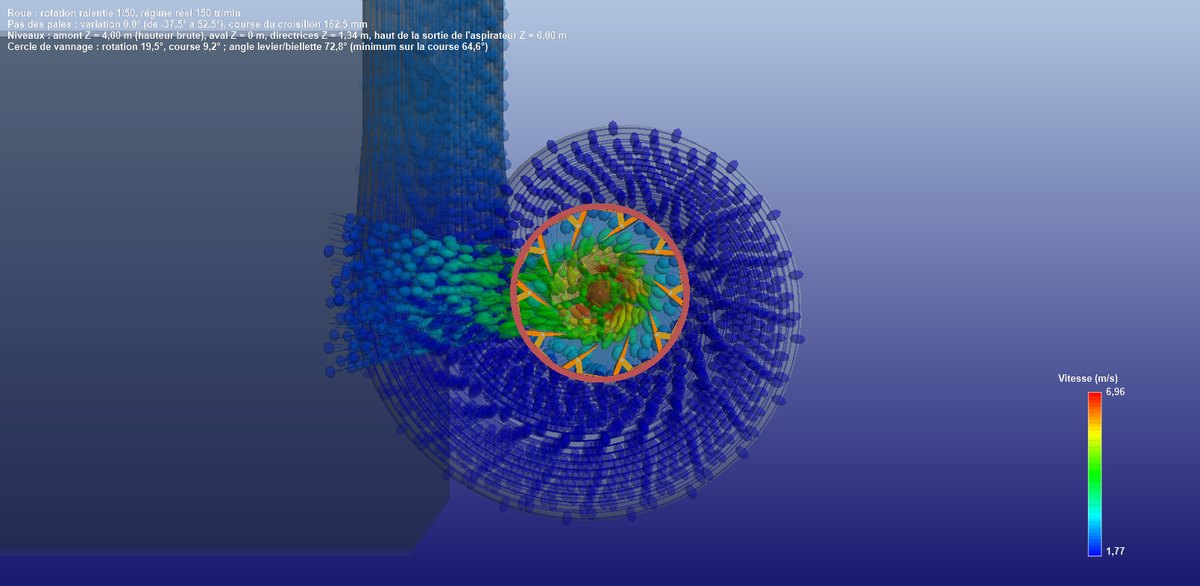
The example installation seen from above in 3D: the spiral casing, the distributor, the runner, and the water trajectories coloured by velocity, blue in the spiral, green at the runner.
2: Implantation: the site, the penstock and the height H2
The Implantation tab receives what you impose: the gross head Hb between the surfaces of the upstream and downstream reservoirs, the maximum flow of the site, and the inlet penstock (length, diameter, roughness chosen from a list of materials). Heliciel derives the section, the velocity in the penstock, the friction head loss by the Colebrook formula and the gross power ρ·g·Q·Hb.
The height H2 places the runner outlet above the downstream level. It governs the pressure at the runner outlet, hence the cavitation risk; Heliciel refuses a value lower than the length of the bulb. When the draft tube length and H2 require it, a horizontal junction tube and an elbow are added to the water path, with their losses.
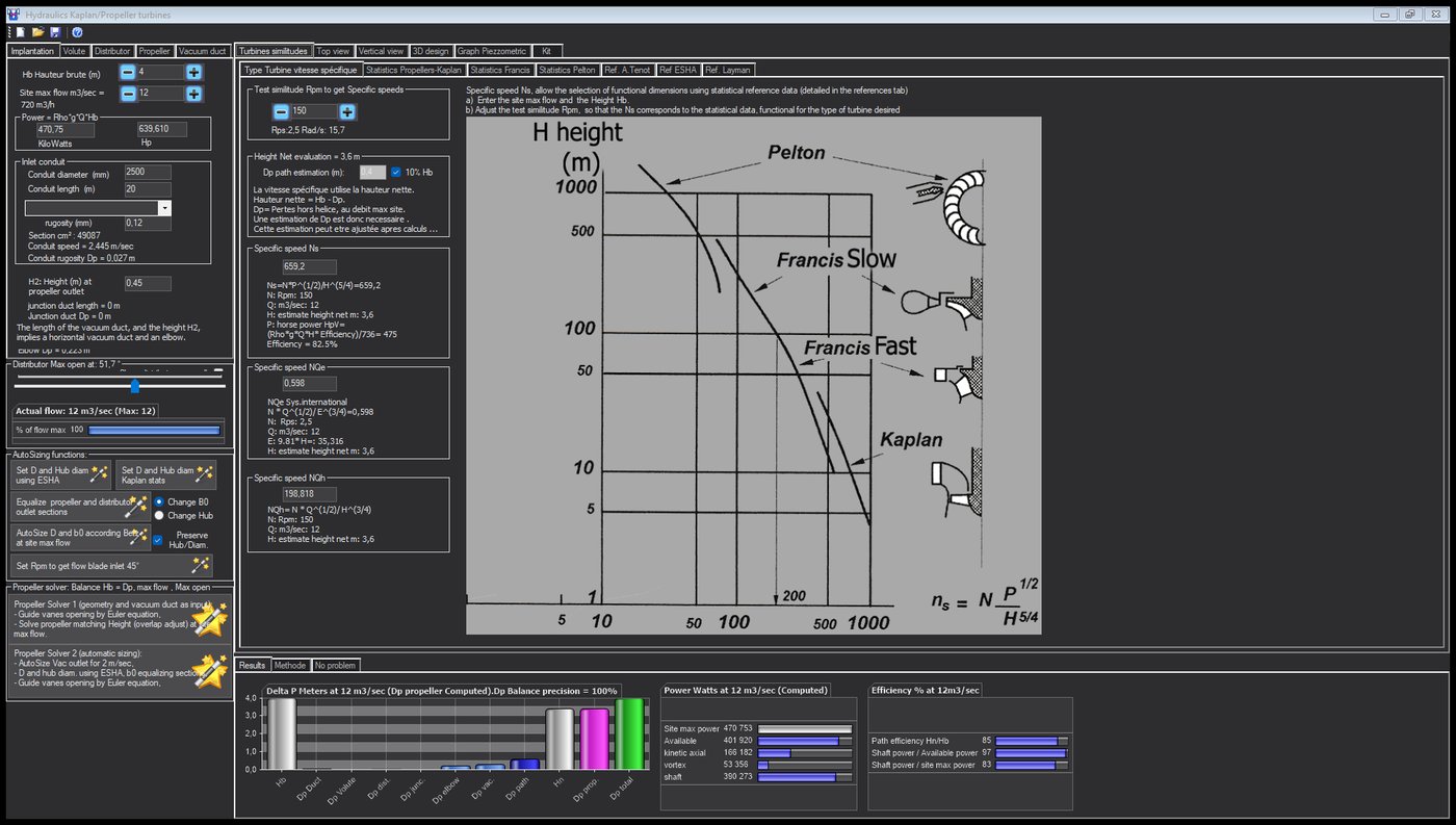
The Implantation tab of the example: 12 m³/s under 4 m, 470.8 kW gross, a 20 m, 2,500 mm penstock run at 2.45 m/s. On the left, the automatic sizing functions and the two solvers.
The values of the example are those of a study case: 12 m³/s and 4 m are the site of the tutorial series; the penstock and H2 are editorial choices, stated as such.
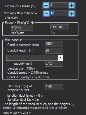
The layout input panel.
3: Specific speed: which turbine family for your head
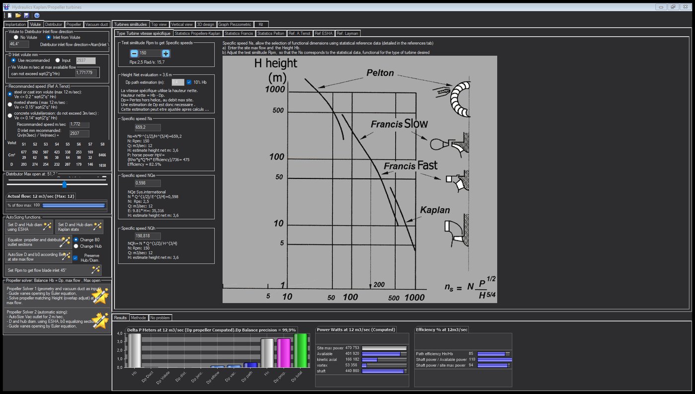
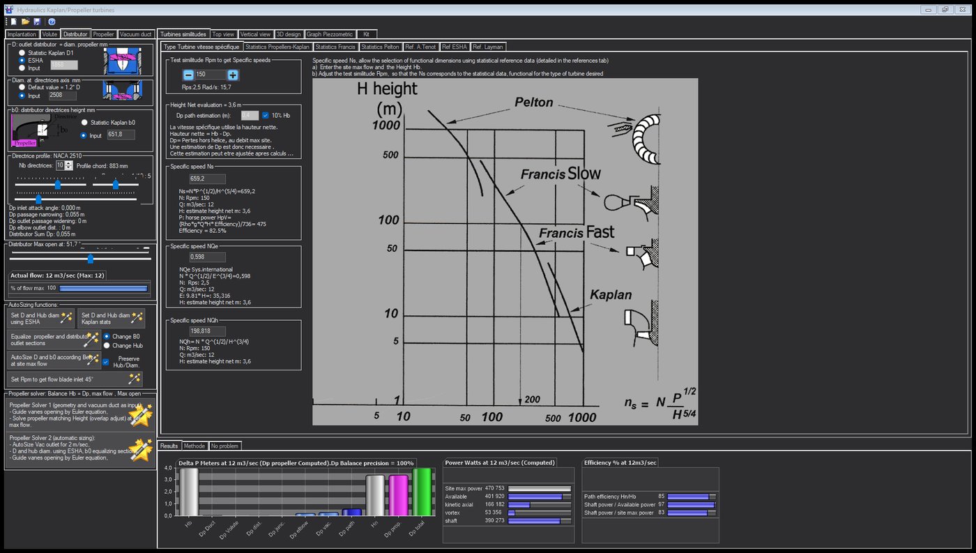
The Type Turbine vitesse spécifique tab computes three specific speeds, Ns, NQe and NQh, from the flow, the net head and a trial speed. The net head is estimated here: Hb minus an estimate of the losses (10% of Hb by default, or your value), which you readjust after a first computation. These numbers are the language of the trade: they tell whether your head-flow pair calls for a Pelton (high head, low flow), a Francis (medium head) or a propeller / Kaplan (low head, high flow).
The adjustment is made through the trial speed: you vary it until Ns enters the Kaplan range (350 to 2,000 in the window). On the example, 150 rpm give Ns = 659. This trial speed becomes the runner speed if you leave it in similarity mode.
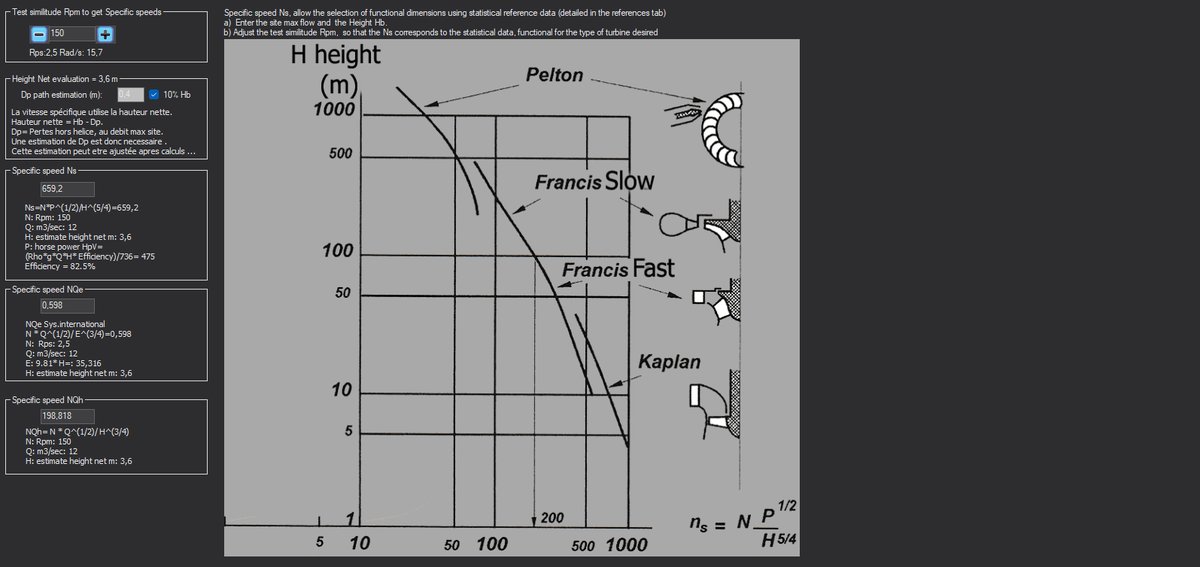
At 150 rpm under an estimated 3.6 m net, Ns is 659: the machine is a Kaplan. The chart locates the three families.
4: Kaplan, Francis and Pelton statistics and references
Three tabs plot, as a function of Ns, the similarity factors recorded on built turbines: for Kaplan turbines the peripheral speed factor ξ₁, the ratio b0/D1 (distributor height over runner diameter) and the ratio d/D1 (hub over runner); for Francis turbines ξ₀, ξ₁ and b0/D1; for Pelton turbines ξ₀ and the ratio D0/d0 of the wheel diameter to the jet diameter. The dimensioning relations are displayed next to the curves: U1 = ξ₁·√(2·g·Hn), D1 = 60·U1/(π·N), then b0 and d from their ratios, and for Pelton turbines the number of buckets and the bucket proportions.
These are fleet trends, useful to know whether a preliminary design is plausible, not guarantees. The Ref. A. Tenot, Ref ESHA and Ref. Layman tabs show the documents these charts are taken from: the Tenot chart, the ESHA guide to small hydropower and the Layman guide, which can be consulted in the window. This is what lets you cite a source in a report.
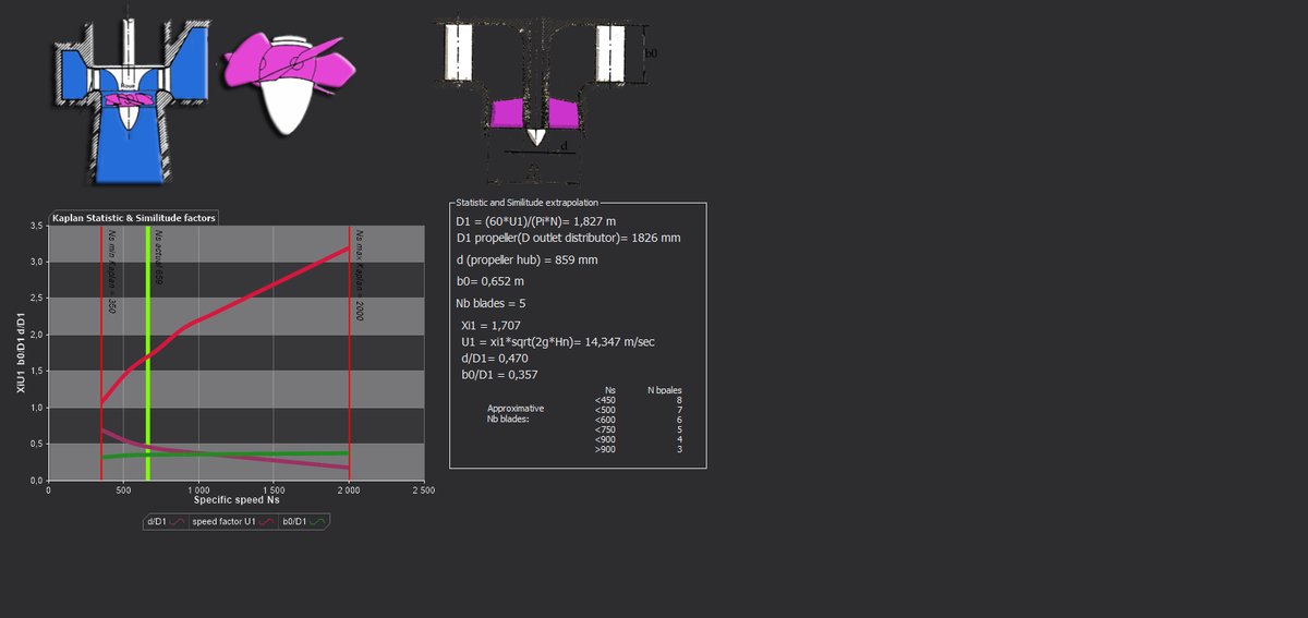
The Kaplan statistics: the three factors as a function of Ns, the bounds of the family, and the dimensions derived for the example.
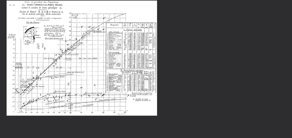
The Tenot chart, zoomable, from which the statistics come.
5: Volute: the spiral casing and its velocity
The Volute tab sizes the spiral inlet. You choose the casing material, and Heliciel proposes the matching allowable velocity (ref. A. Tenot): Ve ≤ 0.2·√(2·g·Hn) for cast iron or steel, 0.15 for riveted plate, 0.14 for concrete, which erodes above 3 m/s. The inlet diameter follows from the flow, or you enter it. Heliciel then computes the eight sections S1 to S8 of the spiral, which keep the velocity constant all around the distributor, and the direction of the stream at the guide vane inlet. A casing that is too small wastes head for nothing; too large, it costs civil engineering.
The Volute tab: cast iron casing, 1.77 m/s recommended at maximum flow, inlet diameter and sections S1 to S8.
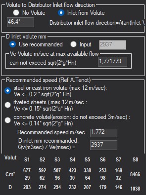
The volute panel: material, admissible velocity, inlet diameter.
6: Distributor: guide vanes, height b0, opening and losses
The distributor is the regulating component of the machine, the one that adapts the flow to the resource of the moment, and the one that gives the water the rotation the runner needs. The Distributor tab carries its whole geometry:
- the outlet diameter D of the distributor, equal to the runner diameter: entered, Kaplan statistics from Ns, or ESHA formula;
- the diameter of the pivot circle of the guide vanes, 1.2 D by default;
- the height b0 of the guide vanes: entered, Kaplan statistics, or equalization of the distributor outlet section with the annulus swept by the runner, b0·π·D = π·(D² − d²)/4;
- the number of guide vanes, their four-digit NACA profile (thickness, camber, camber position) and their opening, on a slider.
Heliciel computes the head loss of the distributor in four terms, after Idel'cik: the angle of attack at the guide vane inlet, the narrowing of the passage, the widening at the outlet and the outlet elbow towards the runner. The sum is displayed under the profile. You also read the passage velocity, the throat radius and the circulation constant K of the free vortex the distributor produces: this is what becomes the swirl sent to the runner.
The Distributor tab of the example: ten guide vanes, b0 652 mm, pivot circle 2,508 mm, opening 51.7°, total loss 0.055 m.
A trap to know: if the pivot circle stays in entered mode with the value of another project, the guide vanes can end up inside the runner. On the example, a 594 mm circle inherited from a micro-turbine, for a 1,574 mm runner, gave 29 m/s at the passage and immediate cavitation: setting it back to default mode restored everything.
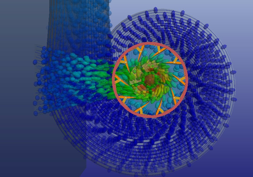
Close-up of the distributor from above: the guide vanes, the gate ring, and the blue particles of the casing accelerating, in green, towards the runner.
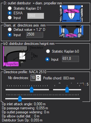
The distributor panel: D by ESHA, axis circle, b0, NACA 2510 profile of the ten guide vanes, and the four loss terms, 0.055 m in total.
7: Propeller: the runner, the speed and the balancing solver
The Propeller tab carries the hub diameter (slider, Kaplan statistics, ESHA formula, or equalization of the sections), the number of blades (entered or statistical), the speed (from similarity, or entered) and the blade overlap as a percentage. The overlap is the adjustment variable: it sets the chord width, hence the head the runner absorbs. The Test cavitation on blades box sends the project the true runner outlet pressure as the blade reference; unchecked, the project receives 100,000 Pa.
The automatic sizing functions of the Implantation tab apply here: Set D and Hub diam using ESHA or Kaplan stats set D and the hub from Ns; Equalize propeller and distributor outlet sections equalizes the sections by acting on b0 or on the hub; Set Rpm to get flow blade inlet 45° looks for the speed that gives a 45° flow angle at the runner inlet, swirl included. The Betz button remains for comparison, but its free-stream assumption does not suit a runner in a conduit: the solver does not use it.
The Propeller Solver does the balancing: gross head = water path losses + head absorbed by the runner, at the maximum flow of the site.
- It opens the guide vanes by the Euler equation: the target angular momentum is K = g·(Hb − losses at that opening)/ω, found by bisection on the slider. If the target is unreachable, Solver 2 tries remedies (b0, then pivot circle); otherwise it stops and says so.
- It adjusts the overlap until the runner absorbs the available head, by a repeated BEM computation. If the head is not enough at the minimum overlap, the speed is reduced.
- It judges cavitation after the balancing, on the water path and on the blades, the blades being judged at the runner outlet pressure. The verdict is information: Heliciel corrects nothing on its own.
Solver 1 keeps the geometry and the draft tube you entered; Solver 2 first sizes the draft tube at 2 m/s, the runner by ESHA and b0 by equalization of the sections. On the example, Solver 2 converged in two minutes: static Δp 2.961 m, swirl head 0.453 m, path losses 0.585 m, total 4.000 m for a 4 m gross head, accuracy 100%.
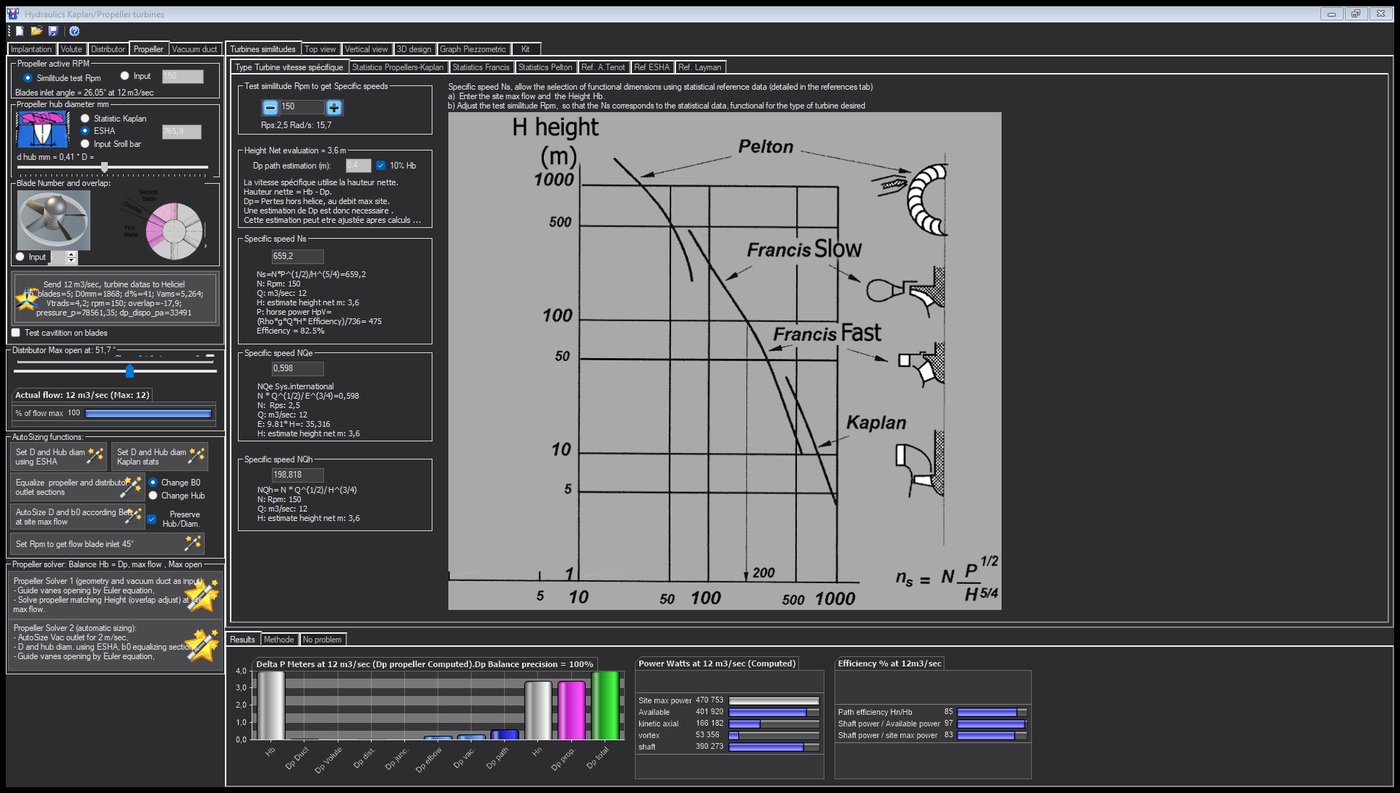
The Propeller tab after balancing: 1,868 mm runner, 766 mm hub, five blades, 150 rpm, overlap −17.9%.
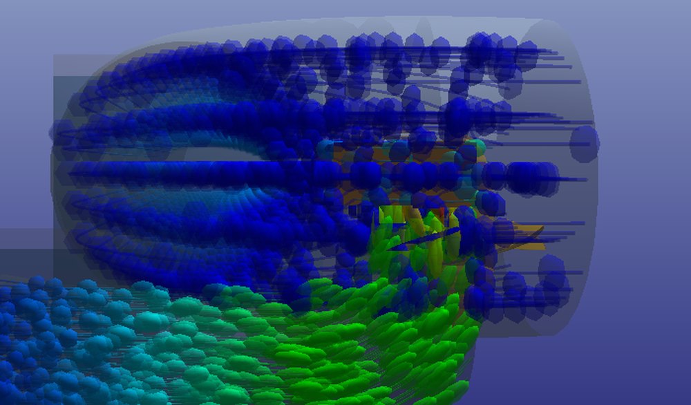
The runner in a cut: the blades, the hub, the guide vanes above, and the particles flowing down from the runner to the draft tube.
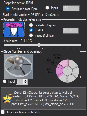
The runner panel: hub, blades, rpm, overlap, cavitation.
8: Vacuum duct: the draft tube and its pressure recovery
The draft tube recovers the kinetic energy left behind the runner: without it, a low-head turbine loses a significant share of its efficiency. The Vacuum duct tab receives its length, its roughness and its outlet section, rectangular, with a height equal to half the width. Heliciel computes the cone angle, the suction gain (V²inlet − V²outlet)/2g, the losses of the cone (Idel'cik up to a 50° total angle, sudden expansion beyond), of friction and of outlet. The AutoSize button sets the section for an outlet velocity of 2 m/s (adjustable) and the length for a 14° cone.
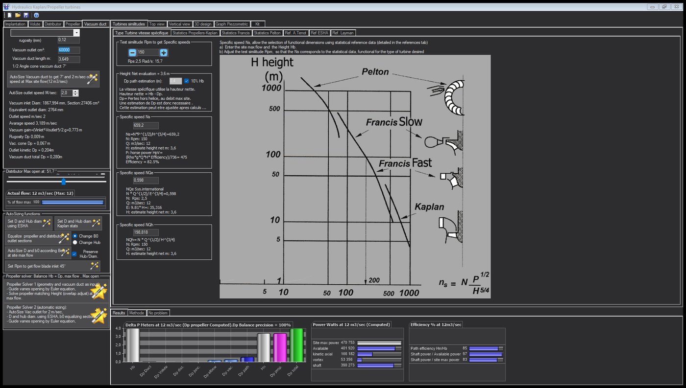
The draft tube of the example: 3.65 m, 6 m² outlet at 2 m/s, recovery of 0.77 m, losses 0.28 m.
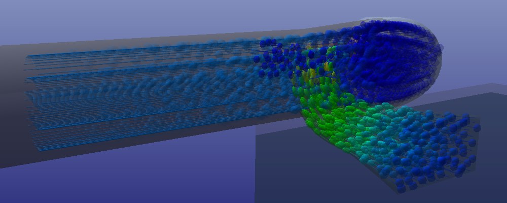
The elbow draft tube with its rectangular outlet, seen from downstream: the trajectories slow down and spread out to the river.
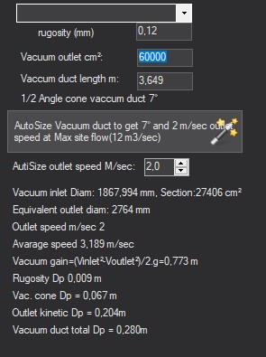
The draft tube panel: length, outlet section, cone angle, gain and losses.
9: Top view, Vertical view and piezometric graph
The two 2D views are the drawings of the installation. Top view draws the spiral of the casing, the guide vane circle and their opening, with details on request (distributor inlet and outlet, guide vane passage, runner inlet, radial sections) and the dotted line of the natural vortex trajectory. Vertical view is the dimensioned meridian section: reservoirs, penstock, guide vanes, runner, bulb, draft tube, with the pressure, the velocity and the section at each point. Wheel and drag move and enlarge the drawing; a button recenters it.
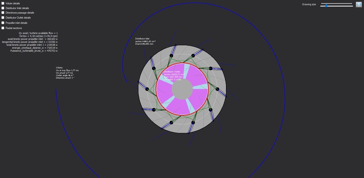
The top view: the spiral, the ten guide vanes, the 4.18 rad/s swirl and the kinetic powers at the runner inlet.
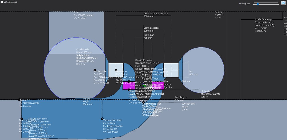
The vertical view: the dimensioned meridian section, from the upstream reservoir to the draft tube outlet below the downstream level.
The piezometric graph is the final check. It follows, from upstream to downstream, the hydrostatic pressure, the dynamic pressure, the gauge pressure, the sum of losses and the total energy, with four markers: the vapor pressure (cavitation limit), the atmosphere, the gross head and the net head. An inconsistency that isolated figures hide shows there at a glance: a pressure that dives below the vapor pressure, a loss that is not where it belongs.
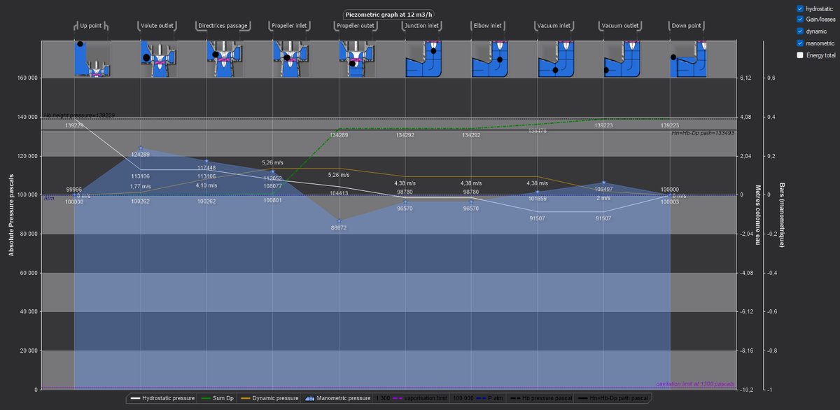
The piezometric graph of the example: the pressure drops at the runner outlet (86.7 kPa) and rises again in the draft tube up to the downstream level.
10: Results, Méthode and Errors: reading the balance and the efficiencies
The Results tab displays three graphs. The heads: each loss of the path, the net head, the runner head and the total, to be compared with Hb. The powers: gross power of the site, available power ρ·g·Q·Hn, axial and tangential kinetic power at the runner inlet, shaft power. The efficiencies: path efficiency Hn/Hb, runner efficiency (shaft power over available power) and overall efficiency (shaft over site).

The results of the example: 390 kW at the shaft for 402 kW available, path efficiency 85%, runner 97%, overall 83%.
Two clarifications on these efficiencies. The available power counts the whole net head, in both its forms: the static pressure and the rotational kinetic energy the distributor gave the water, the swirl. The runner recovers both, and the balance of the window counts its head as the sum of a static Δp and a swirl head, (⟨Vθ²⟩inlet − ⟨Vθ²⟩outlet)/2g. The Heliciel project, for its part, compares the static Δp of its runner with the available head: its ratio of exploited head is therefore the static share, 0.87 on the example, the remainder being converted into torque. Nothing is lost; it is the same balance seen from two windows.
The Méthode tab goes over all of this in the window, step by step. The Errors tab is the last reflex, and the most important one: if it is not empty, the other tabs cannot be read.
11: 3D design: trajectories, cut, exploded view, pitch variation
The 3D design tab shows the whole installation to scale: the upstream reservoir filled up to Hb, the penstock, the spiral casing, the distributor with its guide vanes and their pivots, the computed runner turning slowly, the bulb, the elbowed draft tube with its rectangular outlet and the downstream river whose surface is level with the top of the outlet. The levels are recalled in the legend. Six buttons control the scene:
- Trajectoires fluide: one hundred stream tubes that leave the penstock, wind through the casing, cross the distributor and the runner, then go down the draft tube, with five thousand particles traveling along them at the local velocity. The menu selects the color: the velocity, or the absolute static pressure, computed on each trajectory by Bernoulli from the water path balance. A color scale gives the values.
- Vertical cut: the cut through the vertical plane of the axis, installation, tubes and particles included.
- Show dimensions: the dimensions of the vertical view carried into space.
- Show Turbine: the runner, visible as soon as a design has succeeded.
- Explose: the flat-pattern exploded view, where each component unfolds as flat sheet metal on a plane below the installation, with the maximum deviation between the ruled strip and the true surface.
- Pitch variation: the back-and-forth of the blade pitch angle between its two bounds, driven by the pitch variation mechanism.
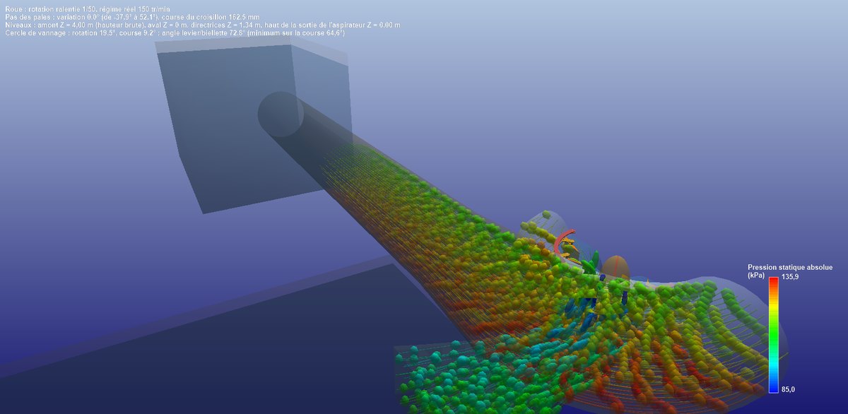
The three-quarter cut, trajectories coloured by pressure: it drops in the casing as velocity rises, falls through the runner, then recovers in the draft tube.
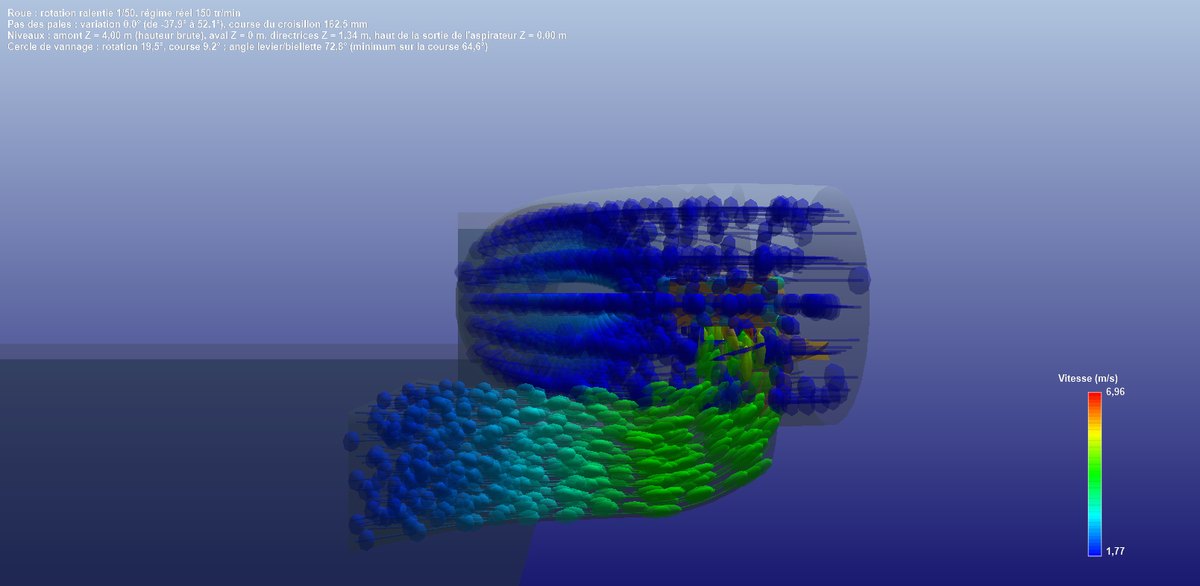
The front vertical cut: the particles swirl in the casing, dive through the 1,868 mm runner and slow down in the 3,649 mm elbow draft tube, below tailwater level.
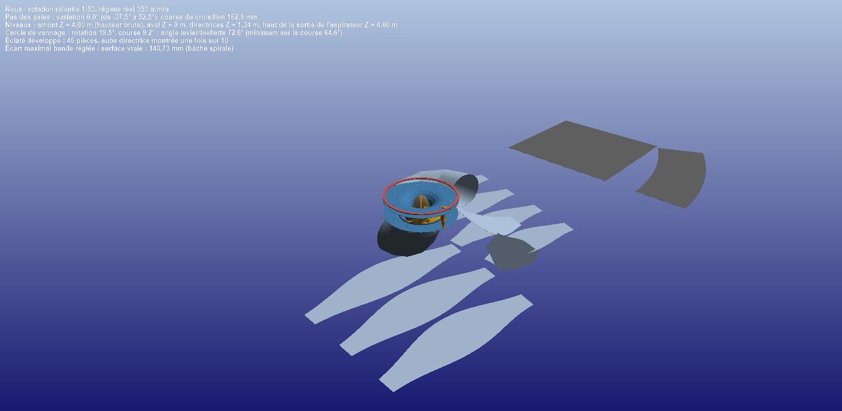
The flat-pattern exploded view: 46 sheet-metal parts unfolded around the distributor and the runner, which stay in place.
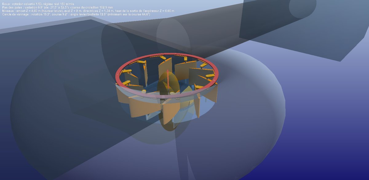
The gate ring and its levers on the guide vanes, and in the transparent hub the spider, the cranks and the links that orient the blades.
The camera is driven with the mouse: rotation with the left button, panning with the right button, distance with the wheel around the target point.
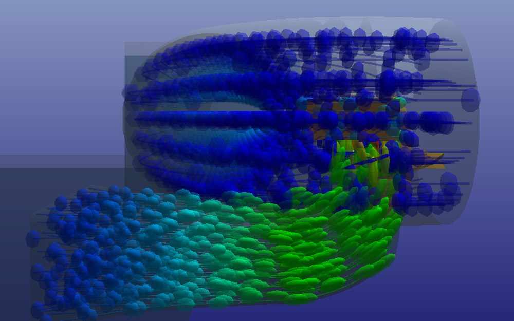
The front cut: the particles swirl in the casing, dive through the runner and slow down in the elbow draft tube.
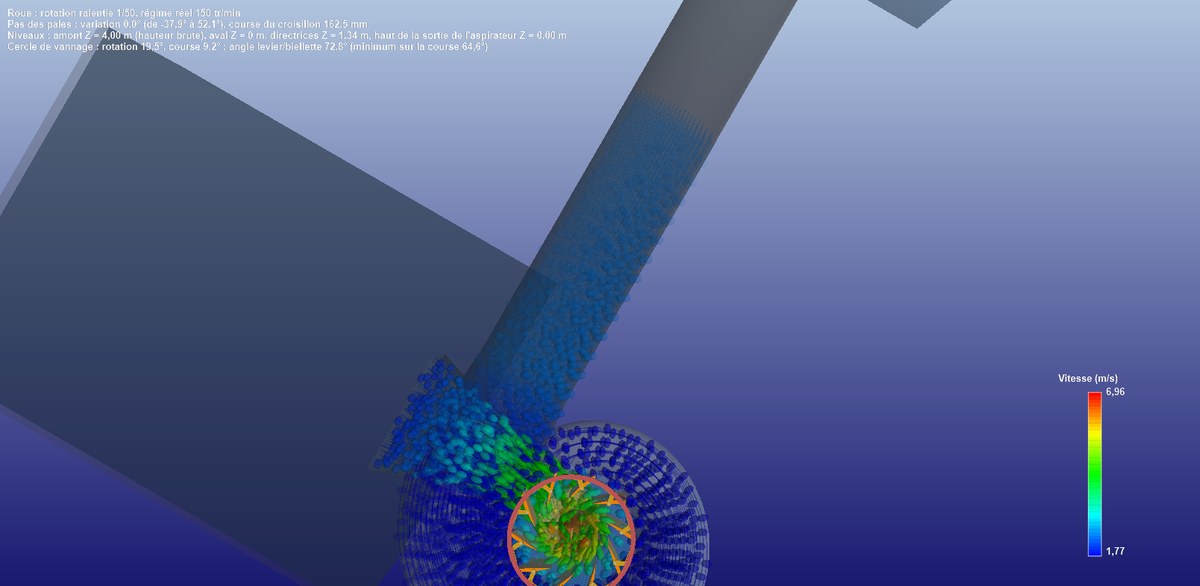
3D top view: the spiral casing carries the trajectories, at constant velocity, all around the distributor.
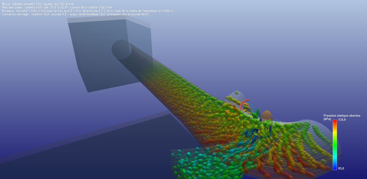
The three-quarter cut, trajectories coloured by pressure: the pressure drops from the casing to the runner, then recovers in the draft tube.
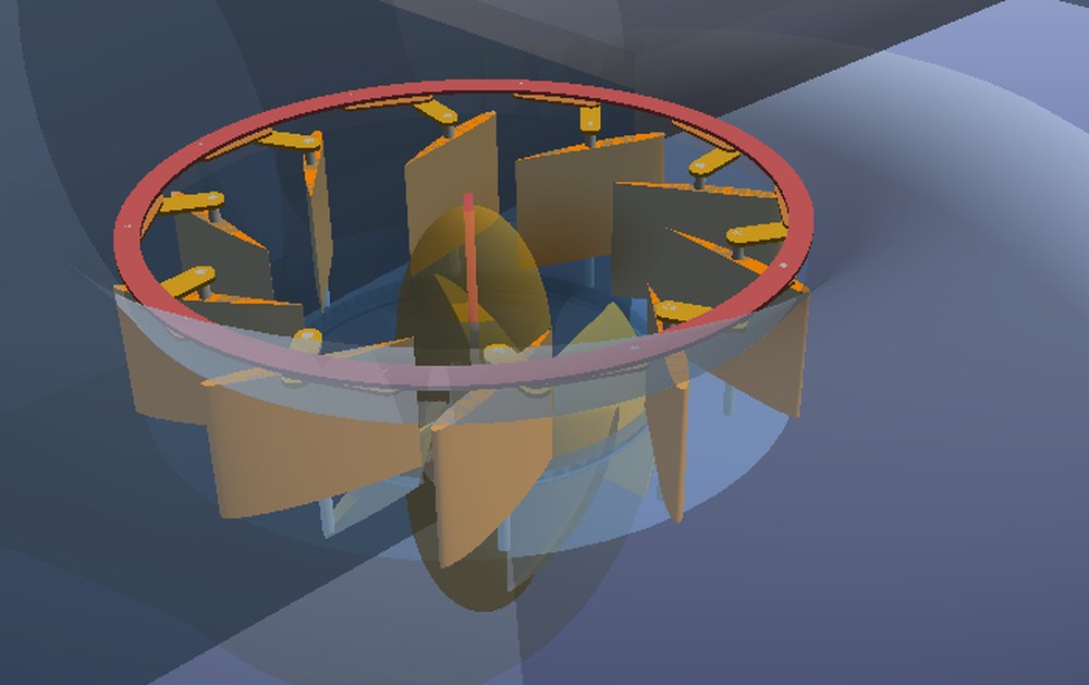
The gate ring, its levers and links on the ten guide vanes, and the pitch mechanism inside the transparent hub.
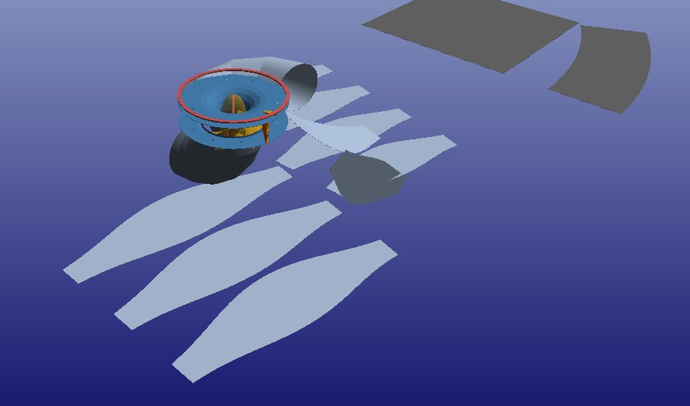
The exploded view up close: the distributor and the runner stay in place, the sheets unfold around them.
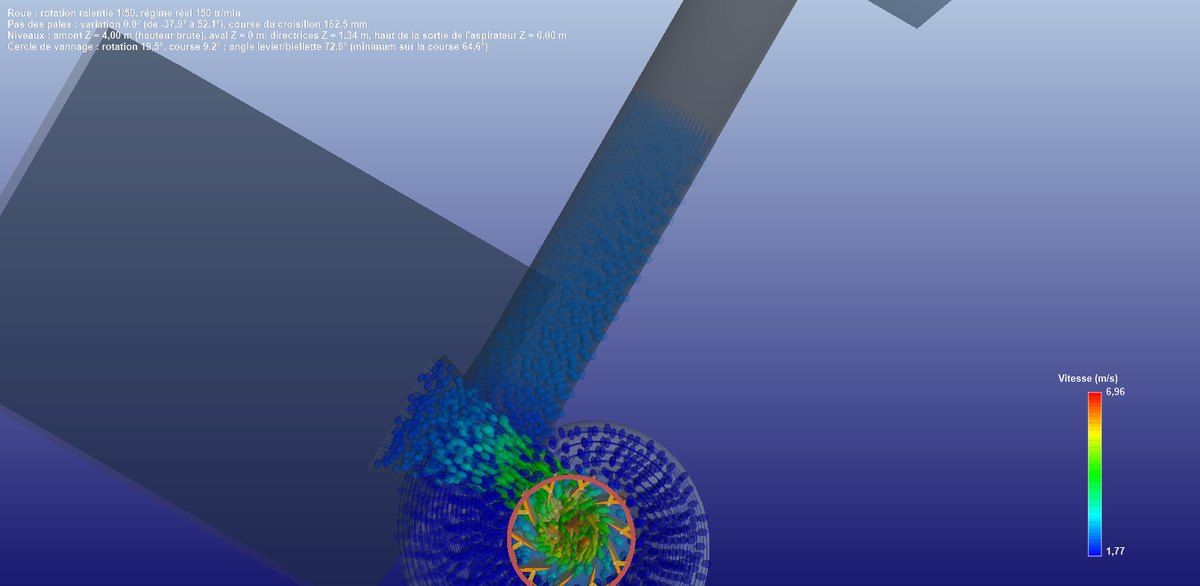
The installation seen from above: the penstock enters the spiral casing, which carries the trajectories all around the distributor.
12: Kit: bill of materials, drawings, gate ring and pitch mechanism
The Kit tab prepares manufacturing. Each component is cut into developable strips: distributor shells, lobster-back segments of the elbow and cone of the draft tube, thirteen sections of the casing, cylinder and connection of the penstock, and a guide vane in ribs, spar and skins. The bill of materials lists each distinct part with its reference, its quantity, the overall size of its flat pattern, its area, its thickness and the deviation between the ruled strip and the true surface; a click on a line displays its dimensioned drawing. An allowable deviation parameter re-cuts the strips of doubly curved surfaces until the tolerance is met, within a limit of two hundred strips per component.
The parameter panel carries the sheet thicknesses of each component (0 = not filled in, and the export is refused) and the dimensions of the two controls:
- the guide vane control, a lever-and-link arrangement: diameter of the pivots, which pierce the flanges and the ribs of the vane, length and angle of the lever, link, radius and section of the gate ring, joints; Heliciel solves the rotation of the ring over the opening stroke and the minimum lever-link angle;
- the pitch variation mechanism of the runner: blade trunnion, crank, link, spider translating in the hub, control rod, azimuthal offset of the joint; Heliciel checks five interferences over the stroke and refuses a kinematic chain that does not close.
The Default linkage values button sets a consistent starting base, derived from the geometry by proportion rules; these are design choices to be reviewed, not a sizing. The export writes to a folder the flat and formed STL of each part, the bill of materials and the clearance holes as CSV; turned and machined parts only have a drawing.
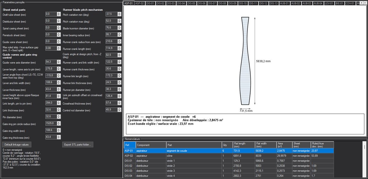
The Kit tab: the panel on the left, the drawing of the selected part, the bill of materials at the bottom.
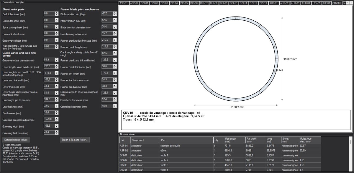
The drawing of the gate ring: a 3,168 mm ring drilled with ten 32.6 mm holes for the guide vane links.
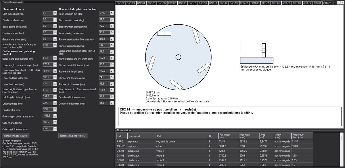
The spider of the pitch mechanism, a machined part: a drawing, no STL.
13: From the .hydt project to the Heliciel project, and on to Mecaflux Pro3D
The toolbar saves and reopens the study in a .hydt file, which carries the settings of the window; reloading replays the computation. The Send turbine datas to Heliciel button writes the runner into the designer project, through its controls: number of blades, diameter, hub, inlet velocity, speed, chords, penstock mode, available head and upstream swirl. The .hlc project is saved separately, and it is the one you take to the CFD bench or to the export of the turbine to Mecaflux Pro3D, where it becomes an element of a gravity network.
To go further, we can follow the complete tutorial of the 12 m³/s case, reread the design method of a Kaplan turbine, or start from a more modest site with the 238 mm Kaplan micro-turbine.
 Global site map
 Mecaflux
 Tutorials Mecaflux Pro3D
 Tutorials Heliciel
 Tutorials Heliciel PRO CFD
 Mecaflux Store
 Compare software functions
 Quotes, Orders, Payment Methods
 project technical studies