
Four B-series propellers imposed on Heliciel in reverse-engineering mode, and their K_T, K_Q and efficiency compared with the published polynomials over the whole J sweep.
Validation: NR640 aircraft propeller (NACA Report 640)
The B-series in Heliciel
Reading Kt, Kq and J
Reverse engineering
Survey: AI with or without Heliciel MCP
Validating Heliciel against published data: the Wageningen B-series
A propeller design program is only useful if you know what to compare its results with. The Wageningen B-series is the best documented family of marine propellers: dozens of geometries tested in the towing tank, whose thrust and torque coefficients were condensed into regression polynomials by Oosterveld and van Oossanen, reproduced by Carlton (Marine Propellers and Propulsion, Table 6.6). Heliciel carries these geometries and these polynomials. This page does the only thing worth doing: impose the geometry of series propellers on Heliciel, have it compute their performance over the whole advance-coefficient sweep, and lay the computed curves over the published ones.
| Propeller | K_T: mean deviation | K_Q: mean deviation | Efficiency: mean deviation | Peak efficiency (Heliciel / reference) | Zero thrust (Heliciel / reference) |
|---|---|---|---|---|---|
| B4-70, P/D 1.00 | +18 % | +22 % | −0.016 | 0.684 / 0.695 | J 1.010 / 1.062 |
| B3-50, P/D 1.00 | +14 % | +17 % | −0.014 | 0.734 / 0.723 | J 1.009 / 1.087 |
| B4-70, P/D 0.60 | +17 % | +18 % | −0.001 | 0.561 / 0.536 | J 0.583 / 0.651 |
| B4-70, P/D 1.40 | +12 % | +13 % | −0.006 | 0.761 / 0.756 | J 1.310 / 1.490 |
1: The question, and what it does not cover
The question is: on an identical geometry, does Heliciel's BEM (Blade Element Momentum) model recover the coefficients measured in the towing tank? The comparison is made over a J sweep, not at one point: a single point may agree by chance, the shape of three curves cannot.
What it does not cover, and has to be said first:
- the B-series is tested without cavitation, as an isolated propeller in open water, at a reference Reynolds number of 2 × 10⁶; Heliciel computes at the local Reynolds number of each element, with the XFOIL polars of the series' segmental sections, and these Reynolds numbers range here from 0.57 to 1.59 × 10⁶;
- the polynomials are a regression of tests: beyond zero thrust they extend a curve but no longer summarise measurements;
- four propellers of the series are compared here: B4-70 at unit pitch in detail, then B3-50, then B4-70 at pitch ratios 0.60 and 1.40, with the same protocol. What follows holds for them, and the protocol can be replayed on the others.
2: The published reference
The K_T(J, P/D, Ae/A0, Z) and K_Q(J, P/D, Ae/A0, Z) polynomials have 39 and 47 terms. Heliciel carries them in its reference module, whose coefficients were checked twice against the scan of Carlton's table. For this page, the same coefficients were ported outside the software, in Python, so that the reference curve depends on none of Heliciel's code; both computations give the same K_T at zero J, 0.4547 for B4-70 at unit pitch and 0.4057 for B3-50, to the fourth decimal.
Detailed propeller: B4-70, P/D 1.00 — four blades, expanded area ratio 0.70, unit pitch. It is the textbook case of the series charts. Reference values for this propeller: K_T at zero J of 0.455, peak efficiency 0.695 at J = 0.842, zero thrust at J = 1.062.
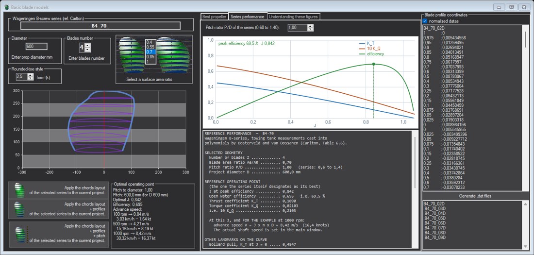 The reference as Heliciel displays it: published curves of B4-70 P/D 1.00, peak efficiency 69.5 % at J 0.842
3: The geometry imposed on Heliciel
The B-Screw Series window applies to the project the chord law, the segmental sections, the thicknesses and the constant-pitch blade angles of the series, in reverse-engineering mode: the geometry is locked as the series defines it, and the software can no longer "correct" it to optimise it. That is the condition of the comparison: we do not compare a propeller designed by Heliciel with the series, we compare Heliciel's computation on the same propeller.
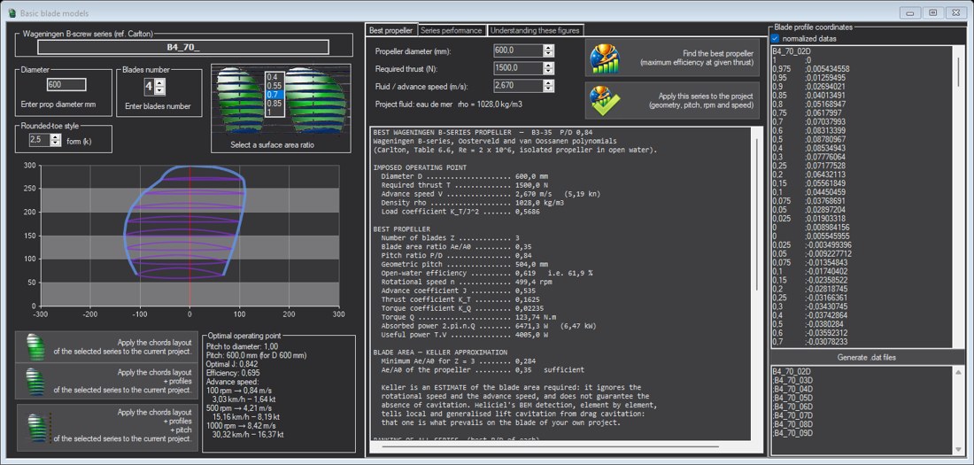 The series selected in the B-Screw Series window: blade outline, optimal point, root section coordinates
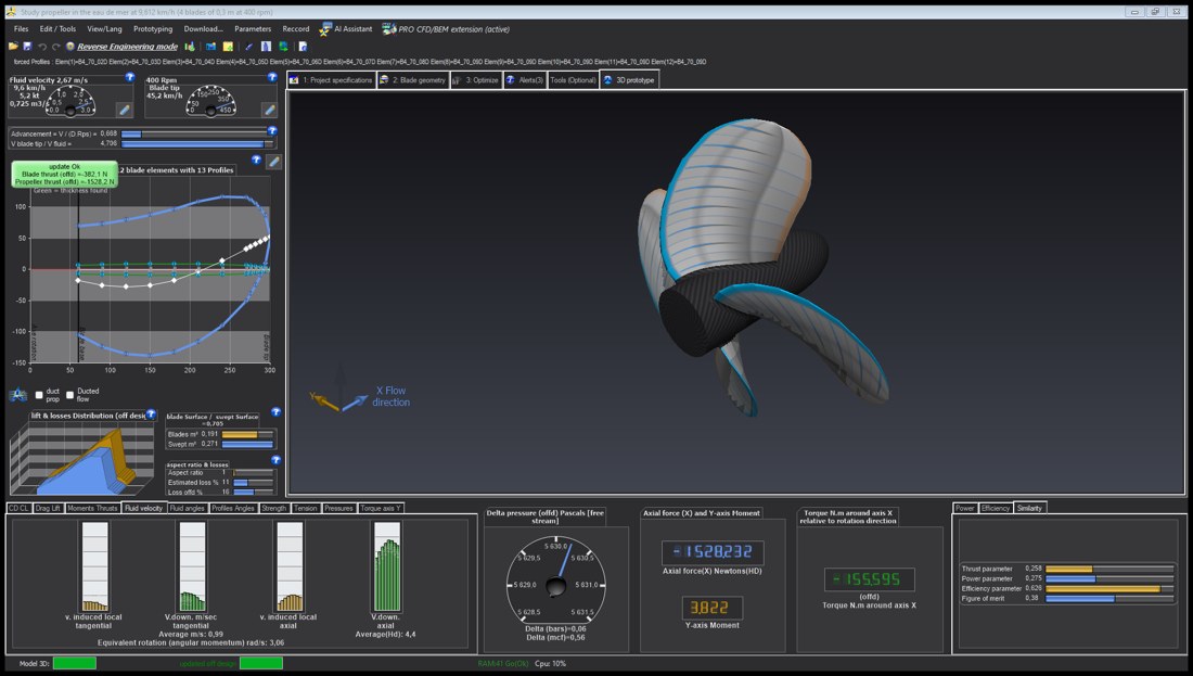 The designer after application: Reverse Engineering mode banner, B4_70 profiles forced element by element
| Parameter | Value applied, read back from the project after application |
|---|---|
| Diameter, hub | 600 mm, 120 mm |
| Rotation speed | 400 rpm (n = 6.667 rev/s) |
| Effective fluid | sea water, 1,028 kg/m³, 10 °C |
| Effective profiles | B4_70_02D to B4_70_09D, forced, one per station of the series |
| Geometric pitch at 0.7 R | 0.600 m, i.e. P/D = 1.00 |
| Blade area | 0.191 m², i.e. 0.68 of the disc (0.70 for the series) |
| Element Reynolds numbers at J = 0.667 | 0.57 × 10⁶ at the root, 1.26 × 10⁶ at 0.55 R, 1.59 × 10⁶ at 0.75 R, 1.38 × 10⁶ at the tip |
The blade angle of each station is that of the series, β = atan((P/D) / (π r/R)), at the radius where the series defines it: 57.86° at 0.2 R, 32.48° at 0.5 R, 24.45° at 0.7 R, 19.48° at 0.9 R, within 0.01° of the theoretical values. The B profiles of Heliciel's database are written with their axis parallel to the face line: the blade angle therefore reproduces the source's face pitch, with no conversion. The computation solves the angle of attack station by station at that same radius, and forms the forces of each element from the two stations that bound it.
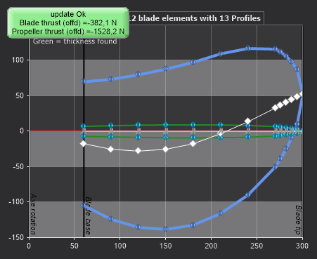 Blade outline and element stations, from root (60 mm) to tip (300 mm)
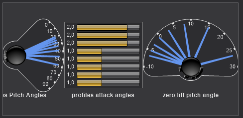 Blade angles (left), element angles of attack at the computed point (centre), zero-lift angles (right)
4: The 3D model, a likeness check
Before any figure, the rebuilt blade must look like a B-series blade: spade outline, broad tip, constant pitch readable in the twist. The views are those of Heliciel's 3D scene.
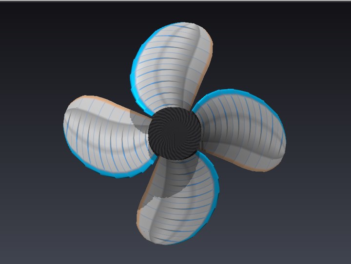 Front view: the four spade-shaped blades of the series
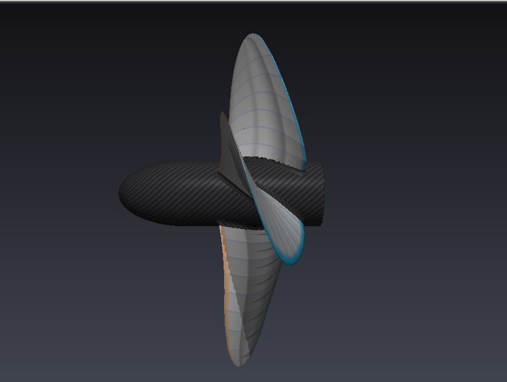 Side view: hub, twist from root to tip
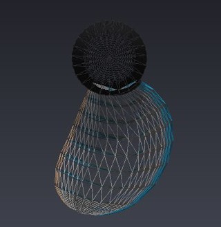 A single blade, as a mesh: outline and sections
5: The J sweep and the comparison, B4-70 at unit pitch
The reverse-engineering operating point is computed, then the multiple analysis sweeps the advance speed from 0.4 to 5.2 m/s at 400 rpm, in 25 points, in off-design mode: the twist is not rebuilt, it really is the series blade that is evaluated at each point. K_T and K_Q are recomputed from the thrust, torque, rotation speed, diameter and density read in Heliciel's table, with the propeller definitions (K_T = T / ρn²D⁴, K_Q = Q / ρn²D⁵).
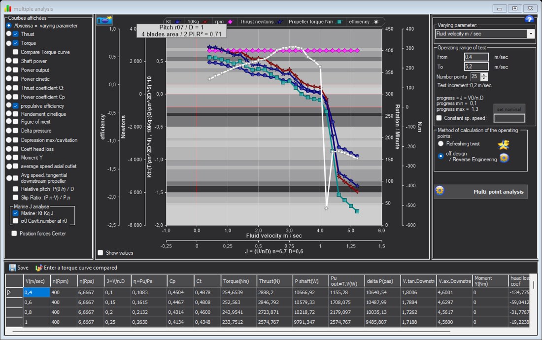 The curves of the Marine: Kt Kq J option of the multiple analysis, as Heliciel plots them
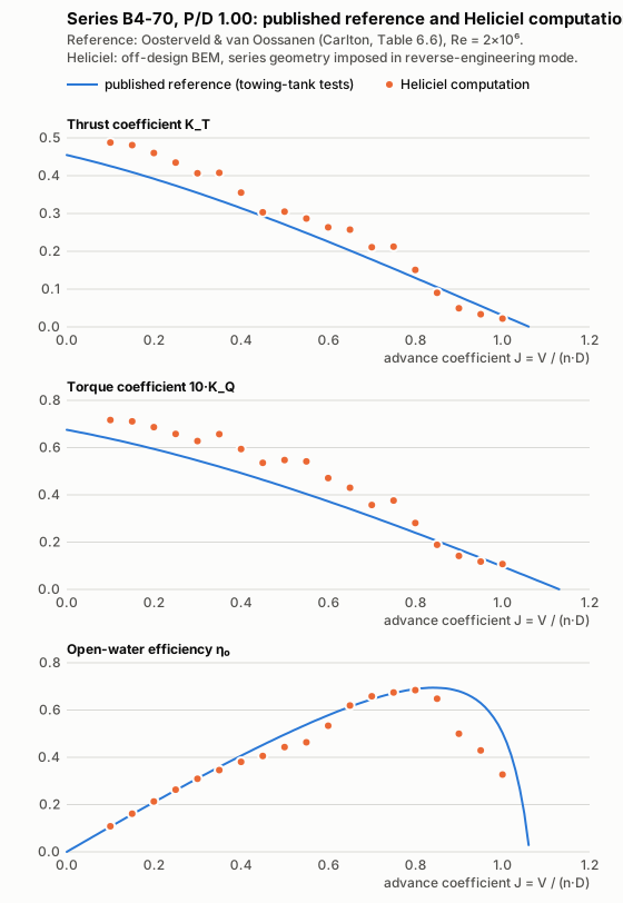 Published reference (blue curves) and Heliciel computation (orange points) on the same J axis
From J 0.1 to 0.8, K_T is overestimated by 18 % on average (from +4 to +38 % depending on the point) and K_Q by 22 % (from +12 to +37 %), while the efficiency follows the reference: 0.684 at best, at J 0.8, against 0.695 at J 0.842. Beyond J 0.85, the computed thrust drops below the reference and vanishes at J 1.010, before the series (1.062): the thrust fall-off as zero thrust approaches is earlier than in the tests. The table of points, from J 0.10 to 1.05:
| J | K_T Heliciel | K_T reference | 10·K_Q Heliciel | 10·K_Q reference | η₀ Heliciel | η₀ reference |
|---|---|---|---|---|---|---|
| 0.10 | 0.488 | 0.425 | 0.717 | 0.638 | 0.108 | 0.106 |
| 0.15 | 0.481 | 0.409 | 0.711 | 0.617 | 0.162 | 0.158 |
| 0.20 | 0.460 | 0.392 | 0.687 | 0.594 | 0.213 | 0.210 |
| 0.25 | 0.435 | 0.374 | 0.658 | 0.571 | 0.263 | 0.261 |
| 0.30 | 0.406 | 0.355 | 0.628 | 0.546 | 0.309 | 0.310 |
| 0.35 | 0.408 | 0.335 | 0.657 | 0.519 | 0.346 | 0.359 |
| 0.40 | 0.355 | 0.314 | 0.594 | 0.492 | 0.381 | 0.407 |
| 0.45 | 0.303 | 0.293 | 0.535 | 0.464 | 0.406 | 0.452 |
| 0.50 | 0.305 | 0.271 | 0.547 | 0.434 | 0.444 | 0.497 |
| 0.55 | 0.287 | 0.249 | 0.541 | 0.404 | 0.464 | 0.539 |
| 0.60 | 0.263 | 0.226 | 0.471 | 0.373 | 0.534 | 0.578 |
| 0.65 | 0.257 | 0.202 | 0.430 | 0.341 | 0.619 | 0.614 |
| 0.70 | 0.211 | 0.178 | 0.357 | 0.308 | 0.658 | 0.646 |
| 0.75 | 0.212 | 0.154 | 0.376 | 0.274 | 0.674 | 0.671 |
| 0.80 | 0.151 | 0.130 | 0.281 | 0.240 | 0.684 | 0.689 |
| 0.85 | 0.090 | 0.105 | 0.189 | 0.205 | 0.648 | 0.694 |
| 0.90 | 0.049 | 0.080 | 0.142 | 0.169 | 0.500 | 0.680 |
| 0.95 | 0.033 | 0.056 | 0.118 | 0.133 | 0.429 | 0.630 |
| 1.00 | 0.022 | 0.031 | 0.107 | 0.097 | 0.327 | 0.504 |
| 1.05 | −0.085 | 0.006 | −0.065 | 0.060 | 2.202 | 0.163 |
6: A second propeller, B3-50, same protocol
To find out whether the deviation belongs to B4-70 or to the computation, the same comparison is replayed on a three-bladed propeller: B3-50, P/D 1.00, three blades, area ratio 0.50, so a clearly less solid blade. Diameter, rotation speed, fluid and sweep are unchanged; only the series changes. Heliciel displays for this propeller a peak efficiency of 0.723 at J 0.869, identical to the Python port of the polynomials.
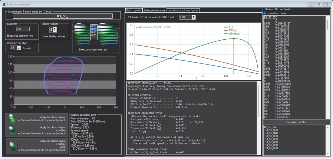 The B3-50 P/D 1.00 reference in Heliciel: peak efficiency 72.3 % at J 0.869
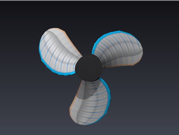 B3-50 applied in reverse-engineering mode, front view
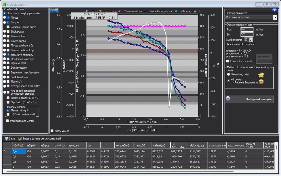 Heliciel's marine curves for B3-50, same sweep as B4-70
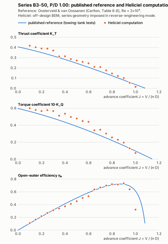 B3-50: published reference (blue curves) and Heliciel computation (orange points)
Same behaviour as B4-70, with a smaller deviation: K_T overestimated by 14 % on average over J 0.1 to 0.8, K_Q by 17 %, efficiency in agreement (0.734 at best against 0.723 for the series). The computed curve is more regular than that of B4-70 up to J 0.9, then the thrust falls off and vanishes between J 1.00 and 1.05, before the reference (1.087). The table of points:
| J | K_T Heliciel | K_T reference | 10·K_Q Heliciel | 10·K_Q reference | η₀ Heliciel | η₀ reference |
|---|---|---|---|---|---|---|
| 0.10 | 0.418 | 0.380 | 0.600 | 0.562 | 0.111 | 0.108 |
| 0.15 | 0.402 | 0.365 | 0.579 | 0.543 | 0.166 | 0.161 |
| 0.20 | 0.390 | 0.350 | 0.566 | 0.523 | 0.219 | 0.213 |
| 0.25 | 0.389 | 0.334 | 0.577 | 0.503 | 0.269 | 0.265 |
| 0.30 | 0.370 | 0.318 | 0.566 | 0.481 | 0.312 | 0.315 |
| 0.35 | 0.313 | 0.300 | 0.512 | 0.459 | 0.340 | 0.365 |
| 0.40 | 0.314 | 0.282 | 0.535 | 0.435 | 0.374 | 0.413 |
| 0.45 | 0.286 | 0.264 | 0.497 | 0.411 | 0.412 | 0.460 |
| 0.50 | 0.273 | 0.245 | 0.479 | 0.386 | 0.453 | 0.505 |
| 0.55 | 0.259 | 0.226 | 0.449 | 0.361 | 0.505 | 0.548 |
| 0.60 | 0.245 | 0.206 | 0.440 | 0.334 | 0.532 | 0.588 |
| 0.65 | 0.210 | 0.186 | 0.341 | 0.307 | 0.638 | 0.626 |
| 0.70 | 0.208 | 0.165 | 0.347 | 0.279 | 0.668 | 0.659 |
| 0.75 | 0.177 | 0.144 | 0.302 | 0.250 | 0.698 | 0.688 |
| 0.80 | 0.145 | 0.123 | 0.256 | 0.221 | 0.719 | 0.710 |
| 0.85 | 0.121 | 0.102 | 0.229 | 0.191 | 0.715 | 0.722 |
| 0.90 | 0.100 | 0.080 | 0.196 | 0.160 | 0.734 | 0.719 |
| 0.95 | 0.054 | 0.059 | 0.128 | 0.129 | 0.639 | 0.691 |
| 1.00 | 0.015 | 0.037 | 0.074 | 0.097 | 0.322 | 0.613 |
| 1.05 | −0.072 | 0.016 | −0.055 | 0.064 | 2.165 | 0.410 |
7: Three pitch ratios on the same propeller, P/D 0.60, 1.00 and 1.40
The B-series covers pitch ratios from 0.6 to 1.4. To find out whether the deviation depends on pitch, B4-70 is replayed at both ends of the series: same blade, same diameter, same rotation speed, only the blade angles change. The sweep is adapted to each pitch so as to cover the reference zero thrust (J 0.651 at pitch 0.6, J 1.490 at pitch 1.4). Deviations are averaged up to three quarters of that zero-thrust J, where both curves are comparable.
| B4-70 | K_T: mean deviation | K_Q: mean deviation | Efficiency: mean deviation | Zero thrust (Heliciel / reference) |
|---|---|---|---|---|
| P/D 0.60 | +17 % | +18 % | −0.001 | J 0.583 / 0.651 (−10 %) |
| P/D 1.00 | +18 % | +22 % | −0.016 | J 1.010 / 1.062 (−5 %) |
| P/D 1.40 | +12 % | +13 % | −0.006 | J 1.310 / 1.490 (−12 %) |
The deviation does not follow pitch: thrust and torque are overestimated by 12 to 22 % at all three pitch ratios, and efficiency follows the reference to the hundredth on average. At pitch 1.4, the computed peak efficiency, 0.761 at J 1.225, matches that of the series, 0.756 at J 1.226. One fact stands out at the same pitch: at the heaviest loadings, up to J 0.35, Heliciel matches the reference (K_T from −3 to +5 %), then the deviation grows with J up to +22 to +34 %. At pitch 0.6 the points are more scattered, from −13 to +32 %: angles of attack are small over the whole range, which amplifies the scatter described in section 9.
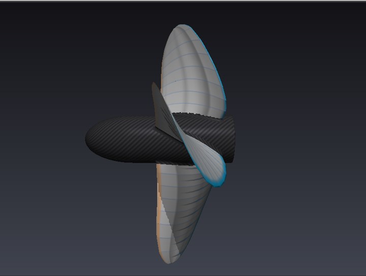 B4-70 at pitch ratio 1.40, side view
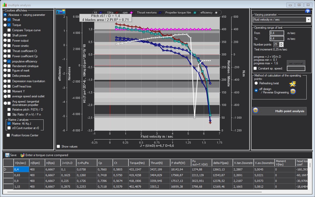 Heliciel's marine curves for B4-70 at pitch ratio 1.40
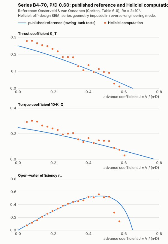 B4-70, P/D 0.60: published reference (curves) and Heliciel computation (points)
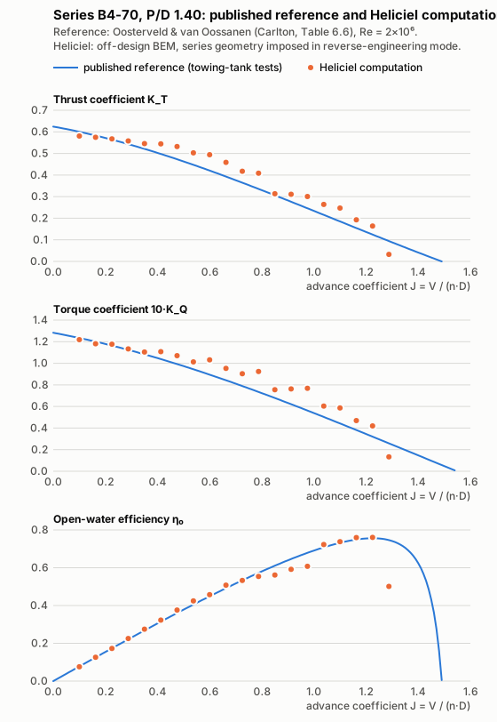 B4-70, P/D 1.40: published reference (curves) and Heliciel computation (points)
Table of points, B4-70 at pitch ratio 0.60
| J | K_T Heliciel | K_T reference | 10·K_Q Heliciel | 10·K_Q reference | η₀ Heliciel | η₀ reference |
|---|---|---|---|---|---|---|
| 0.050 | 0.278 | 0.236 | 0.292 | 0.237 | 0.076 | 0.079 |
| 0.079 | 0.279 | 0.227 | 0.301 | 0.231 | 0.117 | 0.124 |
| 0.108 | 0.265 | 0.218 | 0.295 | 0.224 | 0.155 | 0.168 |
| 0.138 | 0.254 | 0.209 | 0.264 | 0.216 | 0.210 | 0.211 |
| 0.167 | 0.248 | 0.199 | 0.255 | 0.208 | 0.258 | 0.253 |
| 0.196 | 0.232 | 0.189 | 0.241 | 0.200 | 0.299 | 0.294 |
| 0.225 | 0.218 | 0.179 | 0.230 | 0.192 | 0.339 | 0.333 |
| 0.254 | 0.184 | 0.168 | 0.194 | 0.184 | 0.384 | 0.370 |
| 0.283 | 0.184 | 0.157 | 0.201 | 0.175 | 0.414 | 0.405 |
| 0.312 | 0.182 | 0.146 | 0.205 | 0.166 | 0.442 | 0.438 |
| 0.342 | 0.130 | 0.134 | 0.156 | 0.156 | 0.454 | 0.467 |
| 0.371 | 0.107 | 0.123 | 0.135 | 0.147 | 0.466 | 0.493 |
| 0.400 | 0.136 | 0.111 | 0.166 | 0.137 | 0.521 | 0.514 |
| 0.429 | 0.096 | 0.099 | 0.128 | 0.127 | 0.514 | 0.529 |
| 0.458 | 0.114 | 0.086 | 0.148 | 0.117 | 0.561 | 0.536 |
| 0.487 | 0.097 | 0.074 | 0.145 | 0.107 | 0.516 | 0.533 |
| 0.517 | 0.091 | 0.061 | 0.142 | 0.097 | 0.525 | 0.517 |
| 0.546 | 0.028 | 0.048 | 0.089 | 0.086 | 0.276 | 0.482 |
| 0.575 | 0.011 | 0.035 | 0.075 | 0.075 | 0.138 | 0.421 |
| 0.604 | −0.029 | 0.021 | 0.030 | 0.065 | −0.936 | 0.318 |
| 0.633 | −0.100 | 0.008 | −0.037 | 0.054 | 2.753 | 0.150 |
Table of points, B4-70 at pitch ratio 1.40
| J | K_T Heliciel | K_T reference | 10·K_Q Heliciel | 10·K_Q reference | η₀ Heliciel | η₀ reference |
|---|---|---|---|---|---|---|
| 0.100 | 0.580 | 0.600 | 1.219 | 1.234 | 0.076 | 0.077 |
| 0.163 | 0.575 | 0.583 | 1.181 | 1.200 | 0.126 | 0.126 |
| 0.225 | 0.567 | 0.564 | 1.177 | 1.164 | 0.173 | 0.173 |
| 0.287 | 0.558 | 0.543 | 1.133 | 1.125 | 0.225 | 0.221 |
| 0.350 | 0.545 | 0.521 | 1.105 | 1.083 | 0.275 | 0.268 |
| 0.412 | 0.544 | 0.498 | 1.107 | 1.039 | 0.323 | 0.314 |
| 0.475 | 0.532 | 0.473 | 1.070 | 0.993 | 0.376 | 0.360 |
| 0.537 | 0.503 | 0.447 | 1.013 | 0.945 | 0.424 | 0.405 |
| 0.600 | 0.494 | 0.421 | 1.032 | 0.895 | 0.457 | 0.449 |
| 0.662 | 0.459 | 0.393 | 0.953 | 0.843 | 0.508 | 0.492 |
| 0.725 | 0.417 | 0.365 | 0.904 | 0.789 | 0.533 | 0.533 |
| 0.787 | 0.408 | 0.336 | 0.924 | 0.735 | 0.554 | 0.573 |
| 0.850 | 0.313 | 0.306 | 0.755 | 0.678 | 0.561 | 0.611 |
| 0.912 | 0.311 | 0.276 | 0.763 | 0.621 | 0.592 | 0.646 |
| 0.975 | 0.301 | 0.246 | 0.768 | 0.562 | 0.607 | 0.679 |
| 1.038 | 0.264 | 0.216 | 0.603 | 0.503 | 0.723 | 0.708 |
| 1.100 | 0.247 | 0.185 | 0.587 | 0.443 | 0.738 | 0.732 |
| 1.163 | 0.193 | 0.155 | 0.469 | 0.382 | 0.759 | 0.749 |
| 1.225 | 0.164 | 0.124 | 0.420 | 0.321 | 0.761 | 0.756 |
| 1.288 | 0.033 | 0.094 | 0.134 | 0.259 | 0.501 | 0.746 |
| 1.350 | −0.057 | 0.065 | −0.024 | 0.197 | 5.103 | 0.705 |
| 1.413 | −0.154 | 0.035 | −0.254 | 0.135 | 1.364 | 0.591 |
| 1.475 | −0.350 | 0.007 | −0.753 | 0.073 | 1.092 | 0.222 |
8: Bollard pull and reproducibility
Bollard pull. At zero advance speed, the axial momentum equation is loaded the most and the induced velocity alone carries the whole flow through the disc. On B3-50, the off-design computation converges towards a limit as the advance speed tends to zero, with no convergence alert, in 2 to 4 s per point:
| Advance speed | K_T | 10·K_Q | Figure of merit |
|---|---|---|---|
| 0.4 m/s | 0.418 | 0.600 | 0.572 |
| 0.1 m/s | 0.429 | 0.615 | 0.581 |
| 0.01 m/s | 0.438 | 0.629 | 0.586 |
| 0 (the software uses 0.001 m/s) | 0.438 | 0.628 | 0.587 |
The reference gives 0.406 for K_T and 0.596 for 10·K_Q at zero J: +8 and +5 % at bollard pull, in line with the deviations measured at J 0.1. On a drone propeller in hover, the design computation and the off-design computation of the same blade land on the same thrust within 0.2 %: the software's two paths solve the same equation.
Reproducibility. The B4-70 unit-pitch, B3-50 and B4-70 pitch-1.4 campaigns were replayed entirely, from loading the model to the sweep: the 25 points of each are bit-for-bit identical. The computation is deterministic; the irregularities of some curves are not computational noise, they are reproduced identically.
9: What can be said, and what remains open
What is established
- Efficiency holds, forces are overestimated. Up to three quarters of zero thrust, K_T and K_Q are overestimated in similar proportions, by 12 to 22 % on average depending on propeller and pitch, which keeps their ratio, hence the efficiency, close to the reference. For sizing, the consequence is direct: at a given rotation speed, Heliciel predicts on these propellers a thrust and an absorbed power about one sixth too high, for a correct efficiency.
- Thrust vanishes earlier than in the tests. In all four cases, 5 to 12 % earlier in J. Just before, the computed thrust drops below the reference. Too high a pitch would do the opposite: it would push zero thrust towards higher J. The blade-angle convention and the radius where it applies are verified as well (section 3).
- The deviation does not depend on pitch. From P/D 0.6 to 1.4 it stays in the same range (section 7). It does depend on loading at pitch 1.4: nil at the lowest J, growing with J.
- Some curves are irregular, for a known reason. In off-design mode, the angle of attack of each station is searched in whole-degree steps, and blade angles are compared to the nearest degree. Where elements work at only 1 or 2° of incidence, a one-degree jump changes the lift by a noticeable fraction. This rounding is not biased: at the eight stations of B4-70 at unit pitch it ranges from −0.48 to +0.49°, −0.02° on average. It scatters the points around the curve, it does not shift its mean.
- Blade area is not in excess. Related to the disc as in the series, it is 0.68 against 0.70 for B4-70.
- Beyond zero thrust, nothing to compare. There Heliciel computes a windmilling propeller, with forces 8 to 25 times those the regression extends. The regression no longer summarises tests there: the deviation cannot be interpreted either way.
What remains open
- The origin of the force overestimation. Leads to investigate, none verified to date: blade solidity, which leaves the domain of isolated-airfoil polars — the deviation is smaller on B3-50, less solid, than on B4-70 at the same pitch (+14 against +18 % on K_T), which points that way without proving anything on two cases; the absence of a hub-loss correction; local Reynolds numbers, lower than that of the tests. No coefficient will be fitted to this deviation: only a demonstrable formulation error would be corrected.
- The deviation's dependence on loading. At pitch 1.4, Heliciel meets the reference at the heaviest loadings and departs from it as J increases. At low J, angles of attack are high and profile lift saturates; that this saturation offsets the overestimation is a hypothesis, not a measurement.
- The early thrust fall-off near zero thrust. It occurs where angles of attack become small, in the region where the whole-degree incidence search is coarsest; the link between the two has not been measured.
10: Reproducing this comparison
Everything can be replayed in Heliciel in a few minutes: File menu, "Water propulsion propeller" model, B-Screw Series window, selection of the series (B4-70 or B3-50, P/D 0.60, 1.00 or 1.40) at 600 mm diameter, application in reverse-engineering mode, 400 rpm, then multiple analysis on advance speed, off-design mode, with the Marine: Kt Kq J box ticked. Through an assistant connected to the MCP connector, the sequence is charger_modele_projet, appliquer_helice_serie_b, calculer_retro_conception, generer_courbes_analyse_multiple (off-design mode), tracer_courbes with the marine option. The reference curve can be read in the Series performance tab of the same window.
Related pages: validation on the NR640 aircraft propeller (NACA Report 640) · the B-series in Heliciel · Kt, Kq and J · reverse engineering of an existing propeller · computation method · AI with or without Heliciel MCP, a survey in figures
 Global site map
 Mecaflux
 Tutorials Mecaflux Pro3D
 Tutorials Heliciel
 Tutorials Heliciel PRO CFD
 Mecaflux Store
 Compare software functions
 Quotes, Orders, Payment Methods
 project technical studies