Blade sections: XFoil pressure and boundary layer Drawing a wing-mast section in Heliciel Sections and pitch angles of a first propeller

see also: Tutorials how to design propeller

Heliciel's profile database, called the "interactive data base", stores the polars of each profile at various Reynolds numbers: this is where Heliciel collects performance data and chooses the profiles of your propeller blade or wing. In it you rank and search profiles, force a profile onto a blade element, draw new profiles and calculate their polars by driving XFoil, a free profile analysis program. This page is the user guide to this database of aerodynamic and hydrodynamic profiles.

In this page:

• Ranking and selecting profiles
• Forcing a profile onto a blade element
• Managing profile databases
• Searching profiles and building custom databases
• Creating and editing a profile
• Calculating the polars of a profile with XFoil
• Fixing the trailing edge and profiles that do not converge
• Pressure curves (Cp) of a profile
• Boundary layer of a profile

1: Ranking and selecting profiles

The profile data for each Reynolds number are stored in a sorting table, in the database tab. When you select a line, Heliciel displays the performance graphs of the profile at the chosen Reynolds number, together with the shape of the profile. To learn more about Cl (lift coefficients), lift/drag ratio, polars and performance, see the page on the profile database.

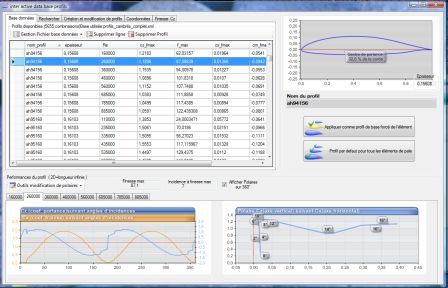
The database tab: the sorting table on the left, the shape of the selected profile at top right, and below it the performance graphs of the profile at the Reynolds number of the chosen line (screenshot of the French interface).

The sorting table ranks the profiles by the criterion of the selected column. For example, to rank profiles by lift/drag ratio (Cl/Cd), click the "finesse" column.

2: Forcing a profile onto a blade element

To make Heliciel use a profile of your choice on one element, you can force that profile for the element selected in the 3D model. Heliciel then uses this profile for the element, whatever the profile selection method in use.

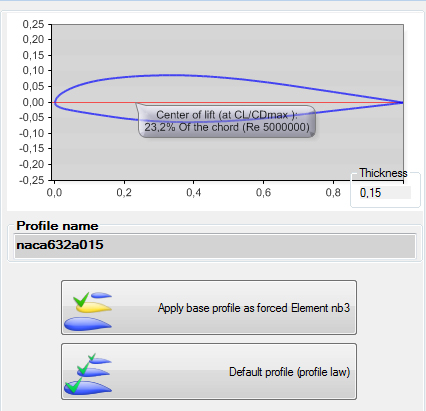
A profile (name and thickness shown below the shape) and the two application buttons, including the one that forces the profile onto the selected element.

3: Managing profile databases

Heliciel uses the loaded database to choose the profiles of your wing or propeller blade. If you want it to favour a category of profiles (flat undersides, symmetrical, NACA...), simply load a database containing only the shapes you want. Everything happens in the File management database menu of the interactive data base.

Using another database. In this menu, choose Open and Use a different database profiles, then select the database you want.

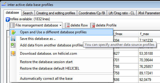
The File management database menu, with its first entry selected and its tooltip.

If the loaded database does not contain the default profile of the project, Heliciel displays a warning message:

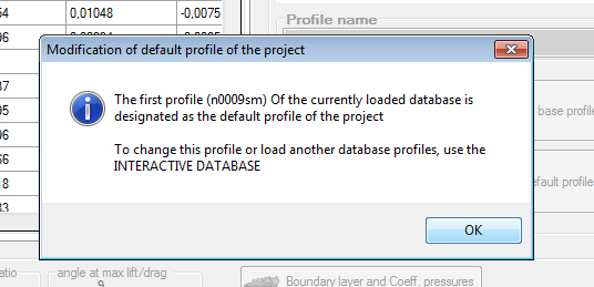
This message tells you that the default profile of your project has changed: Heliciel then designates as the default profile the first profile of the alphabetical list of the new database.

Adding the data of another database. The Add data from another database profiles entry adds two databases together and thereby enlarges the current one. You can then save the current database (Save this database as .. entry) to load it in a future project.

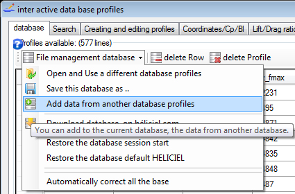
Downloading a database. Download the database from the free Heliciel database download page and save it in the "bases profils" folder of the Heliciel installation folder (for example C:\Program Files\heliciel\Heliciel\bases profils\). In the File management database menu, then choose Open and Use a different database profiles and select the downloaded database. The same menu also offers Download database. on héliciel.com.

This menu also lets you go back: Restore the database session start puts the database back in the state it was in when the software was opened, and Restore the database default HELICIEL restores it as it was at installation. Remove duplicates (marked by _Bis) of the database cleans the database after a merge.

A note on calculation speed. In imposed thickness mode (see the profile selection methods and laws), Heliciel searches the database for the profile whose thickness is closest to the one requested. This search takes a time proportional to the number of profiles in the database. We therefore advise working with small databases.

4: Searching profiles and building custom databases

The interactive data base is where Heliciel collects performance data and chooses profiles. You can modify it, which refines control over profile choices, notably in "Profile law by thickness" mode. For this it is useful to select lists of profiles by criteria of your choice, then create "derived" databases containing your selection. If you save a derived database, you can reuse it later without redoing the selection and sorting. Over the course of your projects you refine your preferred database, and your propeller blades or wings are built automatically with your preferred profiles.

The Search tab is the tool for quickly selecting profiles and creating "custom" profile databases. The diagram below numbers its functions.

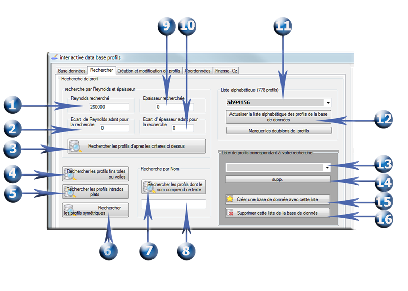
The Search tab, with its sixteen numbered functions. They are detailed in the list below.

The search by criteria works as follows:

1. enter the Reynolds number you are looking for (Reynolds desired);
2. enter the Reynolds gap allowed in the search;
3. start the search by criteria (Search profiles according the criteria above);
4. start a search for thin profiles, of the plate or sail type;
5. search for flat-underside profiles (useful only if you have merged the flat profiles database with another);
6. search for symmetrical profiles;
7. search for profiles whose name includes the text entered in 8;
8. enter the search text;
9. enter the profile thickness you are looking for (Thickness desired);
10. enter the gap allowed for the thickness search;
11. consult the alphabetical list of the profiles in the database;
12. if you have modified the database by adding or deleting profiles or databases, refresh the alphabetical list to take these changes into account;
13. the list of profiles found matches your search;
14. it can be useful to delete the selected line from the list of profiles found;
15. use this list to create a new database (Create a database with the list);
16. remove the list of profiles found from the current database (Delete this list of the database).

These functions let you modify, create and transform your database at will. But you can go further in freedom of profile creation.

5: Creating and editing a profile

The Creating and editing profiles tab gives you complete freedom of creation, provided the shapes remain aerodynamic or hydrodynamic. It lets you create, transform and load a profile, calculate its polars by driving XFoil, then use your creation as a propeller blade or wing profile. Creation takes place in four numbered steps in the tab.

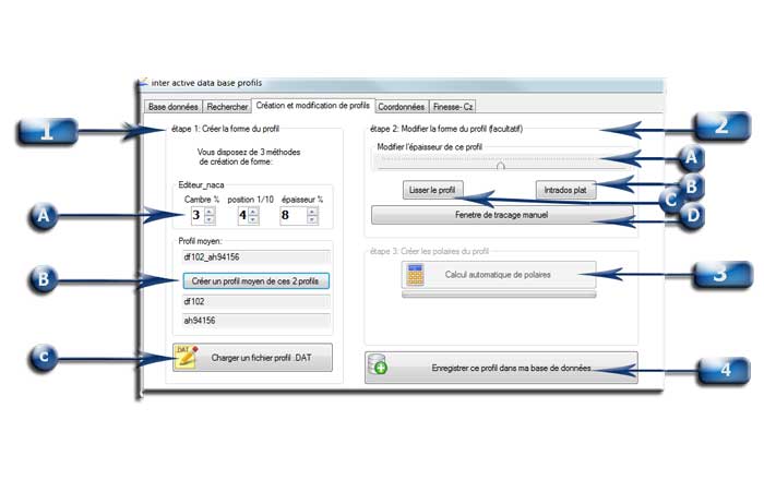
The profile creation tab: step 1 (shape, marks A, B, C), step 2 (editing, marks A to D), step 3 (automatic polar calculation) and saving the profile in the database (4) (screenshot of the French interface).

Step 1: create the profile shape

Three means let you quickly create the starting or final shape of a profile, in addition to the shape selected in the database. You therefore have four ways to create a starting shape.

• A: a NACA 4-digit editor draws the profile by driving the NACA equation (camber, camber position in tenths, thickness).
• B: select two profiles in the database table (click a line in the database tab, then, holding the Ctrl key, a line of another profile).

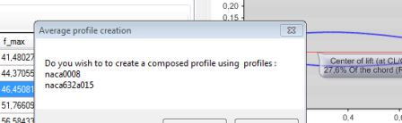
Click "Yes", then click the B button, to merge the shapes of the two selected profiles into an average profile.

• C: import the geometry as a .DAT file (standard profile coordinates file). The profile outline is given by lines of x and y coordinates in two columns. The first data line gives the point 1 in x and 0 in y (the trailing edge), then each line follows the outline up to the point x = 0 via the upper surface, and returns to the point 1.0 via the lower surface. The first line of the file carries the profile name, and the following lines the coordinates.

Step 2: edit the shape (optional)

The shape being edited in the graphics area can be transformed in four ways:

• A: the profile thickness variation slider. Drag it to adjust the thickness;
• B: flatten the underside of the profile;
• C: smooth the profile;
• D: open the profile plotting and correction interface, the plotting and editing profiles window.

Commands A, B and C are also found in the plot window, presented below. It is built into the interactive data base.

The toolbar of the plot window: Apply and close, Close without change, .dat export, Symmetry, Inversion and smoothing menus, and the thickness setting of the upper and lower surfaces.

Various symmetry, inversion, smoothing and thickness tools let you create your profiles to measure, quickly and accurately. All that remains is to start the polar calculation to add your profiles to your performance database. You can also save your drawing in .dat format.

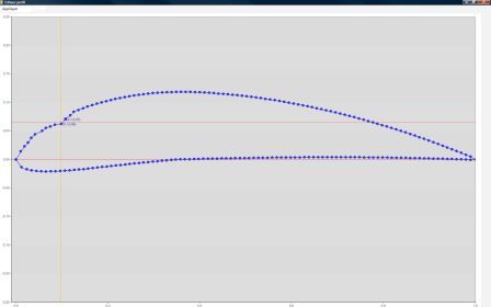
A profile outline drawn with points in the manual plot window.

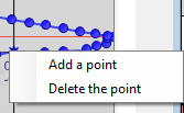
You move the points by dragging them with the mouse, or with the keyboard arrows for maximum precision. A right click adds or deletes a point.

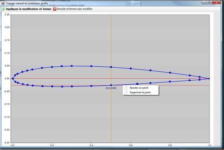
A right click on the outline opens the Add a point / Delete the point menu (screenshot of the French interface).

This creation and correction interface is very useful for preparing coordinate files downloaded from the Internet (for example from the University of Illinois profile coordinates site, UIUC Airfoil Coordinates Database) before the calculation of the polars of the profiles you want to use in your Heliciel projects.

XFoil parameters and paneling

The Xfoil Parameters tab controls XFoil's paneling method. Paneling redefines the distribution of the points forming the profile, and its parameters influence the convergence of polar calculations.

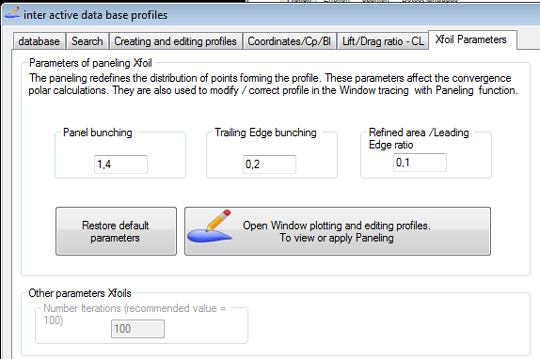
The Xfoil Parameters tab: panel bunching, trailing edge bunching, refined area at the leading edge, the number of iterations, and the buttons to restore default values and to open the plot window.

XFoil's paneling method runs before each polar calculation, but you can also run it from the plot window to correct a profile. It distributes the points so that the angles between the segments of the profile are as small as possible.

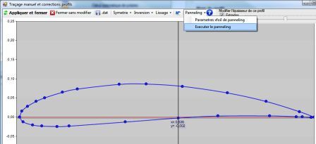
Before paneling: the points are few and irregularly spaced.

Paneling improves the convergence of XFoil calculations, and it also smooths the profile in a refined way.

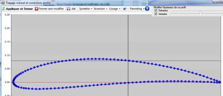
After paneling: the points are more numerous and closer together towards the leading and trailing edges.

6: Calculating the polars of a profile with XFoil

The interactive data base drives XFoil. It injects the geometry of your profile directly to calculate its polars over a range of Reynolds numbers and for the usual angles of attack. Heliciel launches XFoil, then records the results as polars directly in your current database.

The calculation of the polars of a profile can take up to 20 minutes in difficult cases. Plan not to need your PC during that time: interrupting the calculation is possible, but the database is then left in an uncertain state. After a stop before completion, we strongly recommend reloading the session-start database.

The XFoil driving procedure deserves some detail. Heliciel launches XFoil and injects the geometry of the profile you created. Warning: if your profile has shapes too far from an airfoil, XFoil will not be able to calculate it. XFoil does not always converge, which makes it delicate to use. When the calculation of a given angle at a given Reynolds number does not converge, Heliciel slightly changes the Reynolds number or the angle (by 0.1°) to try to reach convergence. This automatic attempt gives far more successes for "difficult" profiles.

After calculating the polar slices between zero incidence and stall, Heliciel extrapolates the performance over 360 degrees, either by adding the performance of flat plates, or by symmetry if the profile is detected as symmetrical. A check and correction of inconsistent data prevents erroneous data from being stored in your database.

Important: XFoil calculates better the performance of profiles that end in a point, whether aerodynamic or hydrodynamic. Some profiles downloadable from the Internet have a poorly tapered, rounded or square trailing edge. Before starting the calculation, check that the trailing edge is well tapered; otherwise XFoil will struggle to converge and will not find all the polars.

7: Fixing the trailing edge and profiles that do not converge

The XFoil calculation can fail for several reasons. One of the most common is too large an angle between two consecutive panels. The plot window displays alerts and information that help to correct the profile. Let us detail what these geometry alerts mean.

Here is an example of a profile with alerts (in red, top left):

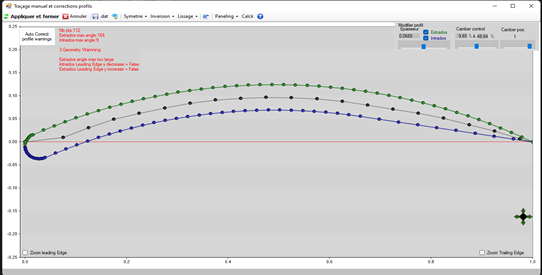
A profile of 112 points. The red alerts at top left flag excessive angles at the leading edge (screenshot of the French interface).

The alerts and information displayed are as follows:

• Nb pts: 112: the number of points of the profile;
• Extrados max angle: 166: the maximum angle between two panels, detected on the upper surface;
• Intrados max angle: 9: the maximum angle between two panels, detected on the lower surface;
• 3 Geometry Warning: when the software detects possible causes of non-convergence, it lists them. Here there are three.

Extrados angle Max too large. If the angle between two consecutive panels exceeds 40 degrees, a warning appears. Here the maximum angle on the upper surface is 166 degrees: beyond 90 degrees, this indicates a step backwards between two upper-surface panels. The problem seems to lie in the order of the points at the leading edge.

Intrados leading Edge y decrease=false. Let us follow the points from the leading edge (x = 0, y = 0) towards the trailing edge (x = 1, y = 0), passing along the underside of the profile, the lower surface. In the zone from x = 0 to x = 0.05 (the leading edge of the lower surface), the y values of consecutive points must decrease. Otherwise, as here, an alert is issued: you must inspect the leading edge points on the lower-surface side.

Extrados leading Edge y decrease=false. The same rule applies along the top of the profile, the upper surface: in the zone from x = 0 to x = 0.05, the y values of consecutive points must increase. Otherwise, as here, an alert is issued: you must inspect the leading edge points on the upper-surface side.

Let us use the "zoom leading edge" and enable the data display to inspect the leading edge of this profile:

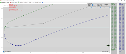
The enlarged leading edge, with the coordinate table on the right: the badly ordered points can be spotted there.

By deleting and replacing a few points, we modify the leading edge to eliminate these alerts:

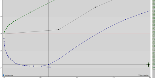
The same leading edge after correction: the points are back in the right order.

Once this is done, paneling distributes the points again:

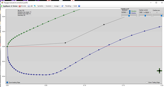
After paneling, the alerts have disappeared and the window reports that the geometry is correct.

This is the profile transformed to converge better. This modification is not only useful for calculation: in reality, excessive angles between panels cause boundary layer separation and reduce lift. These corrections are therefore useful for the profile's proper aerodynamic behaviour.

Example: fixing a poorly tapered or rounded trailing edge

Take the performance calculation of the sg6050 profile, whose coordinates you imported as a .dat file from the same site, excellent and invaluable. XFoil converges on only one or two Reynolds numbers, and your calculated data will not be very useful. Yet the profile looks fine at first glance.

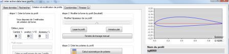
The sg6050 profile imported in the profile creation tab.

Open the manual plot window to edit the profile shape and look at the trailing edge in detail:

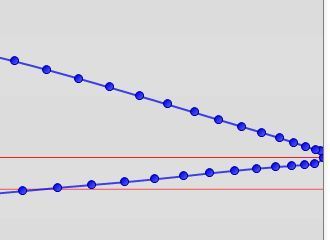
The trailing edge of the sg6050 profile: many points form a rounded end, which prevents XFoil from converging.

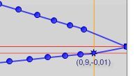
The trailing edge has many points forming a rounded or square end, and this prevents the performance calculations from converging with XFoil. The trailing edge must form a point with no thickness. The plot interface corrects this defect very quickly:

1. delete the surplus points forming the rounded end around the trailing edge, with a right click on the point;

   

2. until the trailing edge ends in a point, like this;

   

3. check that the general shape remains correct, moving any badly placed points if necessary;

   

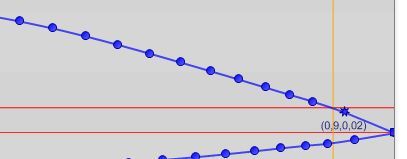
This trailing edge correction considerably improves XFoil convergence, and all your polars can be calculated.

4. All that remains is to save the profile and its performance data in your database, not forgetting to save the database thus modified (Save this database as ..) so you can use it at will later.

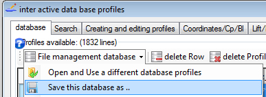
The File management database menu, from which the modified database is saved.

8: Pressure curves (Cp) of a profile

The pressure distribution around a profile tells us about the risk of cavitation, the balance of forces around the profile, and gives an overall view from which to guess the profile's behaviour at the chosen angle of attack and Reynolds number. Editing the Cp (pressure coefficient) curve is an XFoil function, simple to start from the interactive data base: select a line in the list of profiles, then click the Boundary layer and Coeff. pressures button.

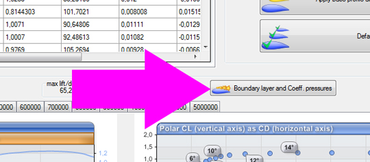
The Boundary layer and Coeff. pressures button (pink arrow), below the profile table, edits the Cp of the selected profile.

XFoil recalculates the pressures with the parameters of the Xfoil Parameters tab. The pressure curve is displayed, and you can then save it.

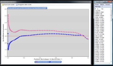
The pressure curve (Cp), from leading edge to trailing edge, with the upper surface in pink and the lower surface in blue. The table of values is on the right (screenshot of the French interface).

The pressures can also be displayed on the 3D model, as a colour code.

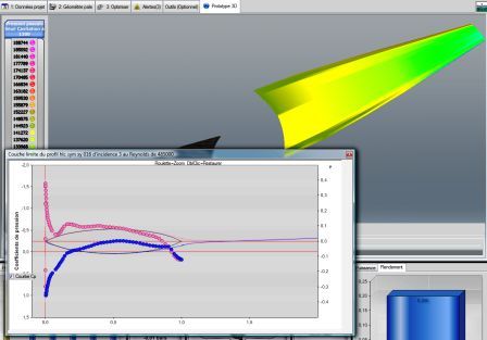
Pressures as a colour code on the blade, with the pressure curve of a non-cavitating profile.

9: Boundary layer of a profile

The same button, Boundary layer and Coeff. pressures, also edits the boundary layer and the pressure coefficients around the profile, at the Reynolds number of the selected polar and for a given angle of attack.

The boundary layer is then displayed in graphical form.

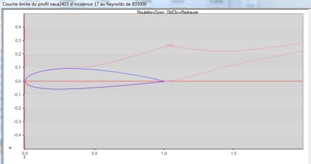
The boundary layer of a NACA 2415 profile at 17° angle of attack, at a Reynolds number of 835,000 (screenshot of the French interface).

The boundary layer and the pressures on the blade can also be edited and viewed in the 3D model tab.

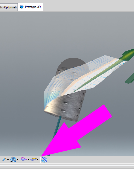
The Prototype 3D tab: the pink arrow points to the toolbar button that displays the boundary layer and the pressures in colour on the blade.

To go further, we can see how Heliciel chooses profiles with the profile selection methods and laws, or download a ready-to-use database from the page on the aerodynamic and hydrodynamic profile database.

Products | Store | My Mecaflux | My Licences | Key generator | My cart | Contact

Copyright © 2024 Mecaflux. All rights reserved. last update 06 february 2024
Terms of sale| Privacy and cookies