
Blade element momentum theory: BEM for wind turbines and tidal turbines
Understand and master BEM theory of blade element for wind turbines and tidal turbines:
Blade element momentum theory is a theory that combines both blade element theory and Froude momentum theory. The Theory of Froude on turbines capture energy "momentum theory" , allowed us to do relation between lnduite axial velocity and thrust force. This theory, assumes that the flow undergoes no rotation, and does not give us indication shape to give our blade..
In reality, the law of conservation of angular momentum requires that the air must have a rotary motion, so that the rotor can extract an outputTorque. In this case, the direction of rotation of flow of the air is opposite to the rotor..Blade element momentum theory, builds on the results of the theory of froude to estimate the elementary axial force (relative to an element), and introduced performance profiles distributed by elements along the blade.The introduction of the rotational movement of air allows the model to better approximate the reality and get the induced velocities tangential and axial component brought by the theory froude using the variation of momentum induced velocity, thus more reliable results. The introduction of performance Cx and Cz profiles allows to determine the geometry and build a real blade.
The theory of the blade element, allows us to define an axial induction factor (a) and a tengentielle induction factor (a '). Solving a sytem equation iteratively converging introducing performance as Cx and Cz of the blade elements, it provides the induced velocities and therefore the performance of the elements.We will also see two corrections, one correcting the fact that the number of blade is considered to be infinite in the method of froude (loss factor blade tip Prandtl) and other correcting the results for the strong values of axial induction, where the Froude theory is no longer valid (Glauert correction for factors greater than 0.4 axial induction)
In developing this model, the following assumptions are considered
- The upstream flow away from the plane of the rotor, is completely axial.
- In the plane of the rotor, the rotational angular velocity ω of the air is, the speed of the rotor reduces considerably far downstream, such that the static pressure far downstream can be considered equal to the atmospheric pressure.
- There is no interference between adjacent components of the blade.
- The flow of air around a part of the blade is considered to be bidimensional..
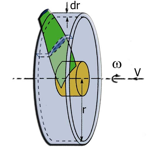
The method of Froude uses variations of momentum in a global volume control, here we use the ring elements as volume control, to know the change in amount of elemental movement, for each ring of the rotor. The sum of the performance of these rings give us the overall performance of the propeller..

- with downstream speed =u1 = V0.(1-a)
- with a factor axial induction

- with tangential velocity downstream C0
- C0=2a'wr (by considering that the tangential velocity upstream is zero)
- with (a '), tangential induction factor
- with r, the distance to the axis (meters), and w the angular velocity(rad/sec)


- the element speed Ve(m/sec) element is perceived by a combination of the tangential speed Omega .r . (1+a') , and the axial velocity V .(1-a)
- The tangential induced velocity is Wt(m/sec)= Omega .r.a'
- The axial speed induced, is Wa(m/sec)= V .(-a)
- Beta(radians) is the pitch angle between the plane of rotation and the profile chord.
- phi(radians) is the angle formed by the rotational speed omega.r and velocity V, upstream of the blade
- Phi+Alphai(radians) is the angle between the plane of rotation of the propeller and the relative velocity Ve.
- Alpha(radians) is the angle view by the profile: Alpha = (Phi+Alphai) - beta
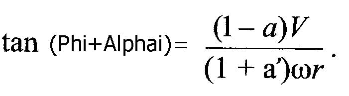
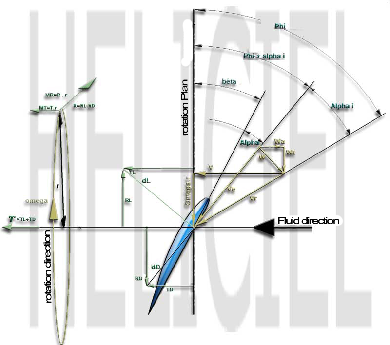 figure2
Remind also that the lift dL, is perpendicular to theelement speed Ve and drag dD. If the coefficients of lift and drag are known drag and lift are defined by
- Lift force dL(newtons) = 0,5. rho. Ve². c .Cl
- Drag force dD(newtons) = 0,5.rho. Ve². c .Cd
- With Cl =lift coefficient extracted from database
- Cd= Drag coefficient extracted from database ,
- c (meters) =profile chord (distance between the leading edge and the trailing edge).
- density kg/m3
- Rotational force(newtons) Pn = dL. cos (Phi+Alphai) + dD. sin (Phi+Alphai)
- Tractive force(newtons) Pt = dL. sin (Phi+Alphai) + dD. cos (Phi+Alphai)
- Cn = CL. cos (Phi+Alphai) + CD. sin (Phi+Alphai)
- Ct = CL. sin (Phi+Alphai) + CD. cos (Phi+Alphai)
- Cn = Pn/(0,5.rho. Ve². c) ( 6.14 )
- Ct = Pt /(0,5.rho. Ve². c) ( 6.15 )
- Ve. sin (Phi+Alphai) =V(1-a) ( 6.16 )
- Ve cos (Phi+Alphai) =wr(1+a') ( 6.17 )
- s(r)= (c(r)B)/(2p r ) ( 6.18 )
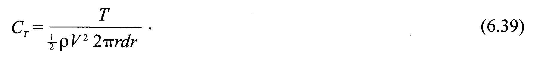
As Pn and Pt are forces per unit length, the thrust T andtorque MR on the volume control of thickness dr is:
- Thrust on element(newtons): T=B.Pn.dr ( 6.19 )
- Torque on element(newtons):MR=r.B.Pt.dr ( 6.20)
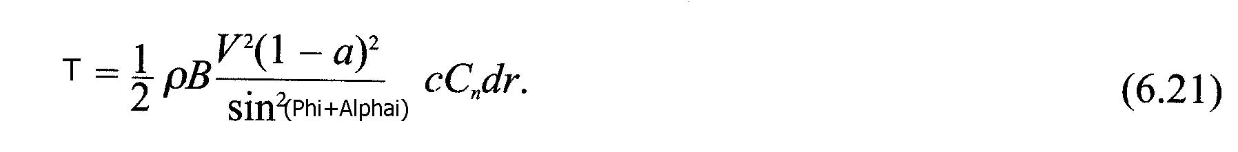
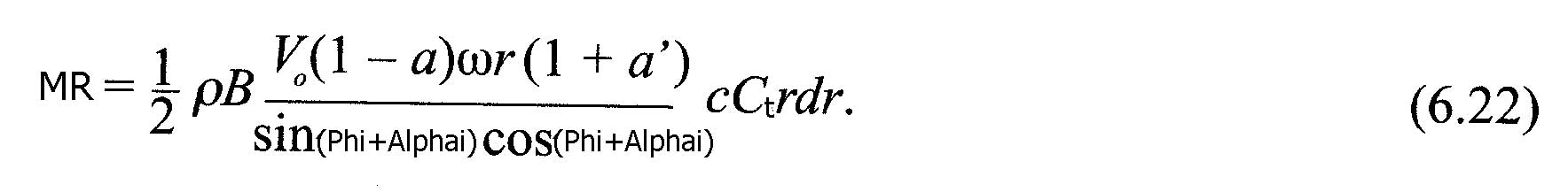
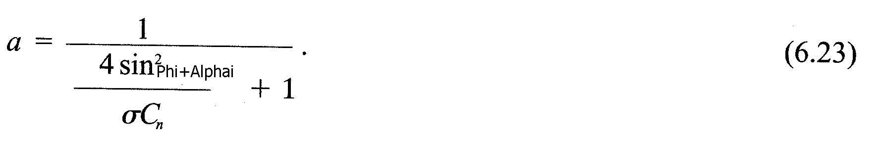
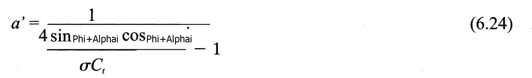
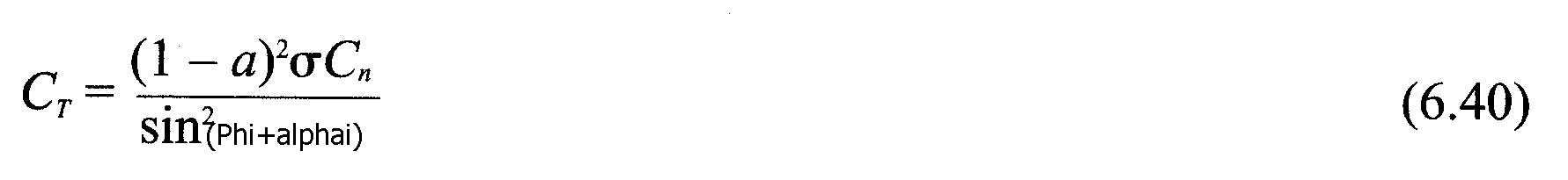
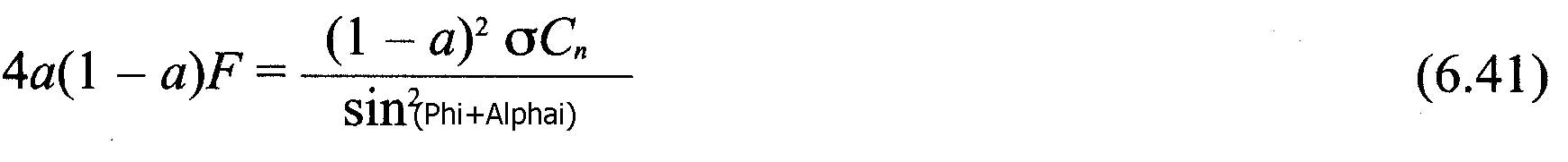
If the two equations (6.21) and (6.4) are equalized, and the definition of solidity is applied,
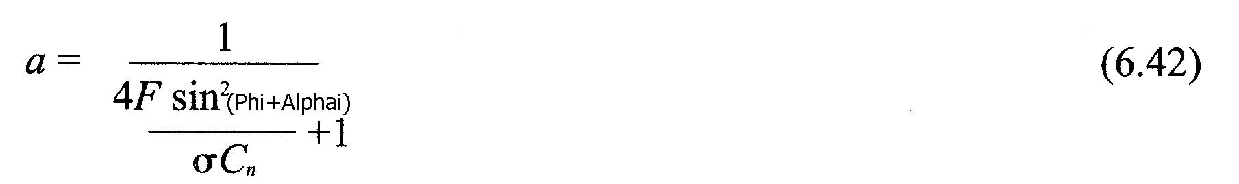
we get the expression of the axial induction factor a:
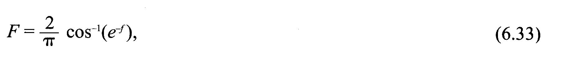
The method froude considered an infinity blade on the rotor disk, the correction factor blade tip losses, derived by Prandtl, is used to correct the performances according to the number of blade.The F factor is used to correct the equations (6.4) and (6.5), so it becomes respectively:


Using equations (6.31) and (6.32) instead of equations (6.4) and (6.5), to establish the equations, factors of axial induction (a) and tangential (a'), we obtain:
Correction high values of axial induction : When the axial induction factor exceeds about 0.4 , the Froude's theory of variations in the amount of movement, is no longer valid. Glauert suggests corrections related to the thrust coefficient. Several empirical relationships between the thrust coefficient Ct, and the axial induction factor, were determined to match the experimental measurements.
We retain that found in Spera(1994) where ac is approximately 0.2.:
- if a <ac:
- if a>ac:


The relations established in this page allow us to create an algorithm converging iterative. It is thus possible to calculate separately the induced velocities, incorporating the corrections Prandtl and Glauert for each blade element. This method uses the performance data profiles. It allows to calculate the thrust and torque on each element.. By adding together these results, the performance of each blade will be found, and the sum of each blade, we will give the overall performance of our propeller..
- HELICIEL uses this method, connected to the database profiles, interactive, for the calculation of propeller energy harvesting, such as wind turbines or tidal turbines..
- initialize a and a ', a = a' = 0.
- calculating the angle (Phi Alpha + i) using equation (6.7)
- calculating the angle of incidence (alpha) in utilsant equation (6.6)
- import data from the performance database for the angle alpha and the profile element
- calculate Ct and Cn following equations (6.12) and (6.13)
- calculate a and a 'after the equations (6.44) or (6.42) and (6.36)
- if a and a 'is changed by more than a certain tolerance, if not complete return to 2
- calculate the forces on the elements
 Global site map
 Mecaflux
 Tutorials Mecaflux Pro3D
 Tutorials Heliciel
 Mecaflux Store
 Quotes, Orders, Payment Methods
 project technical studies