Lifting line: optimal twist of a wing mast Wing and hydrofoil CFD: pressure and lift Sections, geometry, results: the Heliciel method

Prandtl's lifting-line theory explains why a finite-span wing loses part of its lift: air flows around its tips and forms vortices there that push the fluid downwards (the "downwash", or induced velocity). This theory calculates this induced velocity at every point along the span. From it, we obtain the angle of attack the airfoil really experiences, and therefore the true lift and drag of the wing or blade.

In this page:

• Wing-tip vortices and lift loss
• Downwash, induced and effective angle of attack
• Prandtl's lifting-line principle
• Induced velocity of a horseshoe vortex
• Induced velocity formula on the lifting line

Heliciel draws the vortex sheet and the wing-tip losses as follows. The four wings below differ in shape, span and aspect ratio:

Rectangular wing, 2 m span. Aspect ratio = 4, lift-to-drag ratio = 16.	Rectangular wing, 9 m span. Aspect ratio = 18, lift-to-drag ratio = 32.
Tapered wing, 2 m span. Aspect ratio = 5, lift-to-drag ratio = 19.	Tapered wing, 9 m span. Aspect ratio = 33, lift-to-drag ratio = 36.

The higher the aspect ratio, the higher the lift-to-drag ratio. The theory below lets us put numbers on exactly that.

1 : Wing-tip vortices and lift loss on a finite-span wing

As we saw in the page on wings and hydrofoils, lift and drag calculated with the 2D Cl and Cd are theoretical values. They ignore the vortex phenomena of a finite wing, which we now address.

These vortices are born from the pressure difference between the upper surface (suction) and the lower surface (overpressure). At the wing tip, the air from the lower surface tries to reach the upper surface by going around the end.

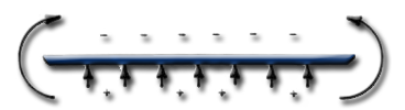
Front view of a wing: overpressure below (+ signs), suction above (− signs), and the resulting flow around the tip (curved arrows).

The same pressure difference creates the lift. We can therefore conclude that the vortex strength, written Γ (gamma), changes with the lift.

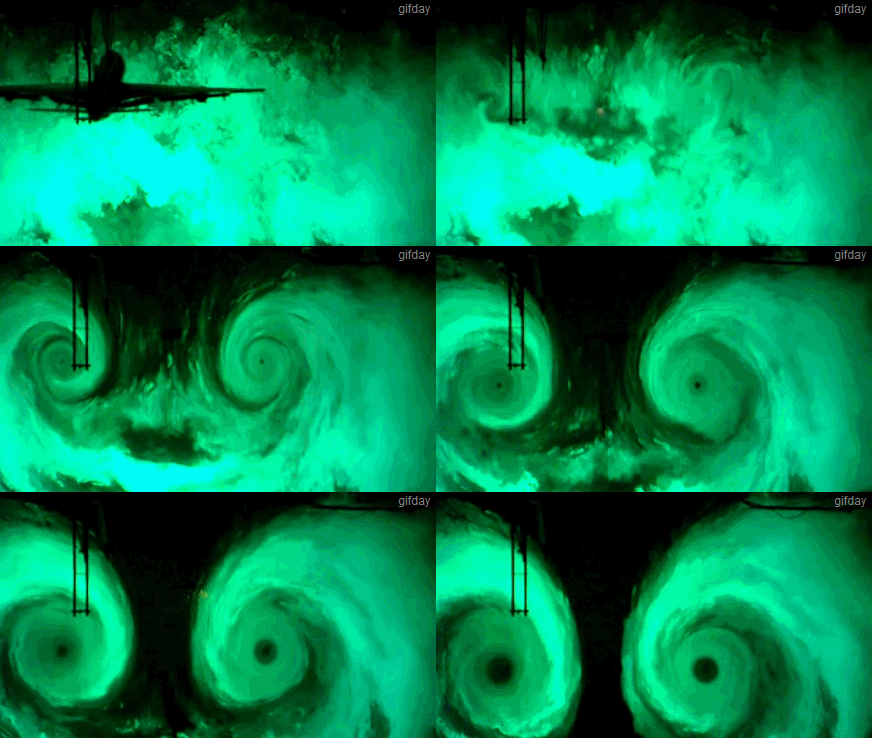
Animation: the lift of the wing generates vortices that roll up behind it.

These vortices change the path of the fluid around the wing and induce downward velocity components. Their value depends on the strength of the vortices and on the distance at which we observe them.

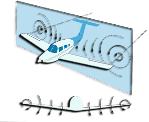
An aircraft seen in perspective, then head-on: the vortices at each tip push the air downwards behind the wing.

2 : Downwash, induced angle of attack and effective angle

Calculating the induced velocities redefines the effective angle of attack of each zone (element) of the wing. With this angle, we can use the 2D performance of the airfoil to calculate lift (dL) and drag (dD) while accounting for the vortices.

Since the induced velocity varies with lift and with the distance from the wing tip, we calculate it for each element of the wing or blade. The next figure shows the change in effective angle caused by the induced velocity at the airfoil of one element.

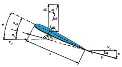
An airfoil on a finite-span wing: the downward induced velocity w turns the velocity seen by the airfoil (from V_∞ to V) and reduces the angle of attack from α to α_eff.

• V_∞ is the upstream velocity, taken at a distance considered infinite, hence undisturbed by the wing.
• w is the velocity induced by the vortices. It points downwards, so we count it as negative.
• α is the geometric angle of attack.
• α_i is the induced angle of attack.
• α_eff is the effective angle of attack, the one the airfoil really perceives: α_eff = α − α_i.

One question remains, and it decides the real performance of our wing: how do we calculate the induced velocities and the effective angle?

3 : Prandtl's lifting-line principle: Kutta-Joukowski, Helmholtz and Biot-Savart laws

In 1918, Ludwig Prandtl developed the first method for analysing a finite-span wing. He replaces all the vortex filaments attached to the wing with a single filament, the "lifting line". Three laws of vortex mechanics are then enough to calculate the induced velocities.

• The Kutta-Joukowski law relates the lift force (in newtons) to the strength Γ of the bound vortex on a wing element of length L (m) immersed in a flow of velocity V (m/s) and density ρ (kg/m³):
  • Lift = Γ · ρ · V · L
  • Γ = Lift / (ρ · V · L)

As a reminder, the 2D lift (in newtons) is: Lift = Cl · element area · ρ · V²/2.

• According to the Helmholtz theorem, a vortex must be closed and cannot end in the fluid. The lift of an element therefore generates a vortex of constant strength Γ, distributed along a line that forms a closed loop.

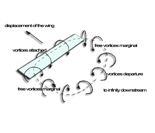
The closed vortex of a moving wing: bound vortex along the wing, two free tip vortices, and the starting vortex left far downstream.

In flight, the "starting vortex", left at infinity downstream, is far enough from the wing for us to neglect the velocity it induces: the velocity induced by a vortex varies as the inverse of the distance to its axis. Only the two free tip vortices remain, with the downward velocity they make the wing feel. They are called semi-infinite because they begin at the end of the element and extend to infinity downstream.

4 : Calculating the induced velocity of a horseshoe vortex

Let us replace the lift force with a line of vortices attached at the centre of pressure of the airfoils (about a quarter of the chord back). It continues as two tip vortices of the same strength Γ. Without the starting vortex, we obtain a horseshoe vortex system.

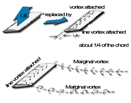
Lift replaced by a line of bound vortices at 1/4 chord, continued by two tip vortices.

This horseshoe system, of constant strength Γ equivalent to the lift, generates downward induced velocities under the wing.

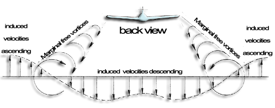
Rear view of an aircraft: under the wing the induced velocities point down (downwash); beyond the tips they point up (upwash).

• The Biot-Savart law gives the induced velocity w (m/s) at a point P located at a distance h from a semi-infinite tip vortex of strength Γ. The lift of the element, known from the Cl of the airfoil, supplies the strength: we can therefore determine the induced velocity −w at point P.

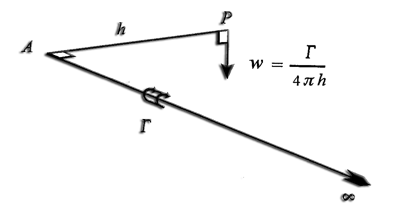
A semi-infinite vortex of strength Γ runs from point A to infinity; at point P, at distance h, it induces a velocity perpendicular to the plane defined by A, P and the vortex.

w = − Γ / (4π h)

The velocity w is negative because it points downwards.

Induced velocity of a single isolated system. Let us place point P on the y axis, between the two free vortices located at −b/2 and +b/2 (b is the span). The induced velocity at y has two terms:

1. −Γ / [4π (b/2 + y)], the contribution of the vortex located at y = −b/2;
2. −Γ / [4π (b/2 − y)], the contribution of the vortex located at y = +b/2.

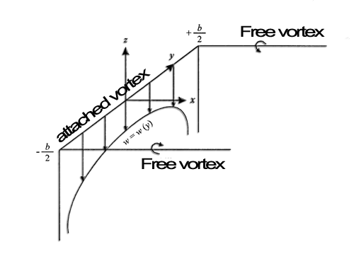
The horseshoe in perspective: bound vortices between −b/2 and +b/2, free vortices downstream, and the curve w(y) of the induced velocity, which plunges towards the tips.

The induced velocity as a function of position y, for an isolated system, is therefore:

• w(y) = − Γ / [4π (b/2 + y)] − Γ / [4π (b/2 − y)]
• which is equivalent to: w(y) = − Γ / (4π) · { b / [(b/2)² − y²] }

In this last expression, the induced velocity tends to minus infinity as y approaches a tip (y = b/2 or y = −b/2). That cannot describe a real wing. Prandtl solves the problem with the lifting-line concept.

5 : Induced velocity and induced angle formulas along the lifting line

Helmholtz's first theorem says that the strength Γ of an isolated vortex is constant and equivalent to the lift. A varying lift, hence a varying Γ, cannot be represented by a single isolated system. Yet lift does vary along the span.

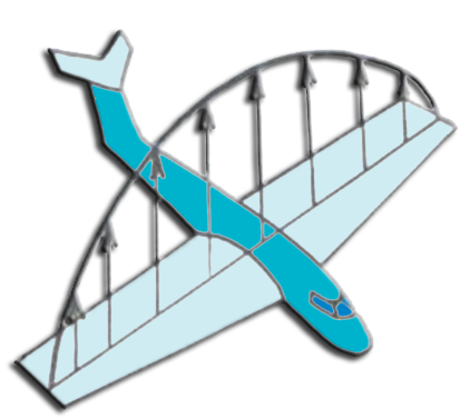
Lift distribution (hence Γ) along the span: highest at the centre, decreasing towards the tips.

Such a variation is only possible if vortex filaments, of strength equal to the variation, join the wing or leave it.

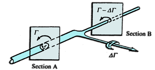
A vortex tube of strength Γ (section A) splits: a filament of strength ΔΓ leaves downstream, and Γ − ΔΓ remains in section B.

A superposition of vortices can therefore represent the change in vortex strength associated with the lift of a wing. At every point where the lift varies, a vortex of strength equal to that variation forms.

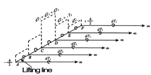
A lifting line discretised into points A to F: at each jump in circulation (dΓ₁, dΓ₂, dΓ₃…), a free vortex leaves towards infinity downstream.

In reality, this vortex sheet forming at the trailing edges merges:

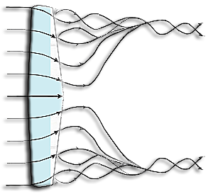
Seen from above: the filaments leaving the trailing edge roll up around one another.

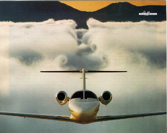
It then forms the two tip vortices that are sometimes visible, for example behind an aircraft flying low.

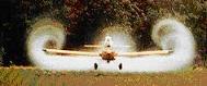
Photograph of an aircraft seen head-on: the tip vortices, made visible by white trails, roll up behind each wing tip.

Because lift varies continuously and gradually, the number of horseshoe vortices of strength dΓ superposed on the lifting line is infinite.

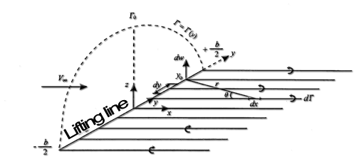
The lifting line, from −b/2 to +b/2, with the circulation distribution Γ = Γ(y) and an elementary free vortex dΓ shed from point y.

• The elementary strength dΓ of the horseshoe vortex corresponding to the segment dy of the lifting line located at y is: dΓ = (∂Γ/∂y) · dy.
• This free vortex of strength dΓ induces a velocity dw at point y₀. The Biot-Savart law, recalled below, gives the velocity induced by a semi-infinite vortex.

Same figure as above: w = Γ / (4π h) in absolute value.

Let us replace Γ with (∂Γ/∂y) · dy and h with y₀ − y. The elementary induced velocity at point y₀, produced by the free vortex of strength dΓ passing at y, is:

dw = − (∂Γ/∂y) dy / [4π (y₀ − y)]

The total velocity induced at y₀ by the whole free vortex sheet, from −b/2 to +b/2, is:

w(y₀) = − 1/(4π) ∫_−b/2^+b/2 [(∂Γ/∂y) / (y₀ − y)] dy

Back to the angle figure: the induced velocity w sets the induced angle of attack.

The induced angle of attack α_i follows from this velocity:

α_i(y₀) = atan [ − w(y₀) / V_∞ ]

Heliciel applies this approach element by element. It thus finds the effective angle of attack, then the real forces on each section, as we describe in Heliciel's calculation method.

References: "Aérodynamique subsonique" by Ion Paraschivoiu, published by the École polytechnique de Montréal. A description of Prandtl's lifting-line theory can also be found on J. Haertig's site (in French): http://j.haertig.free.fr/aerodyn_theorique/index.html, in particular in this PDF document: Prandtl's lifting-line theory.

To go further, we can see how the same idea applies to a rotating blade in the page on the induced velocity of a propeller, or go back to the general page on wings and hydrofoils.

Products | Store | My Mecaflux | My Licences | Key generator | My cart | Contact

Copyright © 2024 Mecaflux. All rights reserved. last update 06 february 2024
Terms of sale| Privacy and cookies